Dataset

Data Source

The data we used is from our client, the UCL Eastman Dental Institute. They provided us with 194 3D teeth models (sextants). They also provided us with 14 real patient teeth models to be displayed in the software.

Originally, we were supposed to train the deep learning model on real patient data. However, due to the ethical issues, we did not recieve the dataset until March 2023. Therefore, we agreed to build a proof-of-concept model using the sextant teeth models, where a sextant is 1/6^th of all the teeth (containing 4 to 6 teeth). Since teeth sextants are only a part of the whole teeth, it is easier for dentists to scan and collect data. We recieved a dataset of 127 3D teeth models on the 13th of March and 67 more on the 23rd of March. We began training and improving our model since then.

Data Description

The data we received is in the PLY file format, which is a format for storing 3D point cloud data. Each teeth model is labeled with a tooth wear grade from 1 to 4 on each tooth manually by experienced dentists. Hence, the label for a tooth model consists of 4 grades. According to the TWES2.0 standard, mentioned in the Research section, the overall tooth wear grade depends on the highest grade among the 4 teeth.

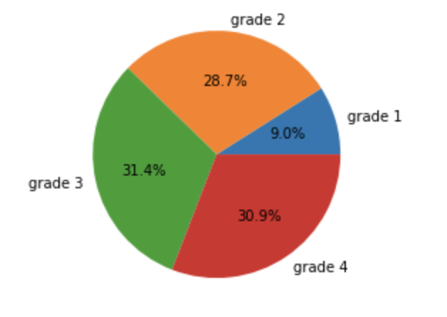
The distribution of the teeth model dataset is shown in the following pie chart.

Fig.1 - Distribution of original dataset

Data Cleaning

After examining the dataset, we found that there are many teeth models that are not labeled correctly, for example some 0's are labeled as "o", some tooth models have more than 4 grades but some have less. Therefore, our first task was to clean the data and rectify the criteria of the labels.

After cleaning the data, we moved on to data augmentation to increase the volume of the dataset.

Data augmentation

As we only received 194 teeth models, which is insufficient to train a deep learning model, we decided to use data augmentation to increase the size of the dataset. Additionally, from the pie chart above, we can see that the dataset is imbalanced, which is not suitable for training a deep learning model. Therefore, we also need to increase the volume of data that has a grade of 1, which is obviously smaller than rest of the groups.

Method 1: Rotation

                        
    # random rotation
    theta = np.random.uniform(0, np.pi * 2)
    rotation_matrix = np.array([[np.cos(theta), -np.sin(theta)], [np.sin(theta), np.cos(theta)]])
    point_set[:, [0, 2]] = point_set[:, [0, 2]].dot(rotation_matrix)

Method 2: Jitter

                        
    # random jitter
    point_set += np.random.normal(0, 0.02, size=point_set.shape)

Method 3: Randomly selected
For each point cloud model, researchers usually select 1024 or 2048 points from a large number of points. The teeth models that we received usually contain 40k to 70k points, which is far more than we need. Hence, we firstly randomly selected 2048 points from each tooth model and we repeated this process to randomly select 2048 completely different points from the point set. As a result we can generate 20-30 different point cloud models from each teeth model.

                        
    # read in the ply file 
    with open(file, 'rb') as f:
        plydata = PlyData.read(f)
    pts = np.vstack([plydata['vertex']['x'], plydata['vertex']['y'], plydata['vertex']['z']]).T

    # randomly choose 2048 points and delete these points from the set
    num_points = np.array(len(pts))
    choice = np.random.choice(num_points, self.npoints, replace=True)
    num_points = np.delete(num_points, np.where(np.isin(num_points, choice)))
    point_set = pts[choice, :]

    # repeat the process according the how many points left
    ...

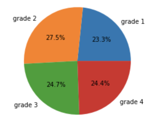
After augmenting the dataset, we increased the number of data that has a grade of 1. The new dataset distribution is much more balanced and is displayed below:

Fig.2 - Distribution of current dataset

Training and Testing dataset

Ratio of training and testing datasets: 80% training, 20% testing

A commonly used ratio of splitting training and testing dataset is training:testing = 8:2 or 7:3. However, our dataset is relatively small and we want to have more data for training to achieve a good result. We decided to use 80% of the dataset for training and 20% for testing.

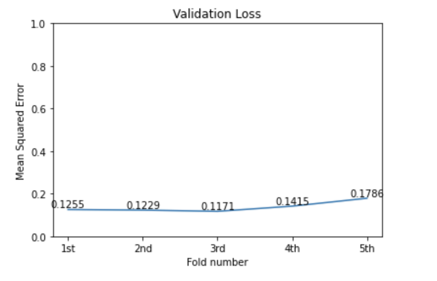
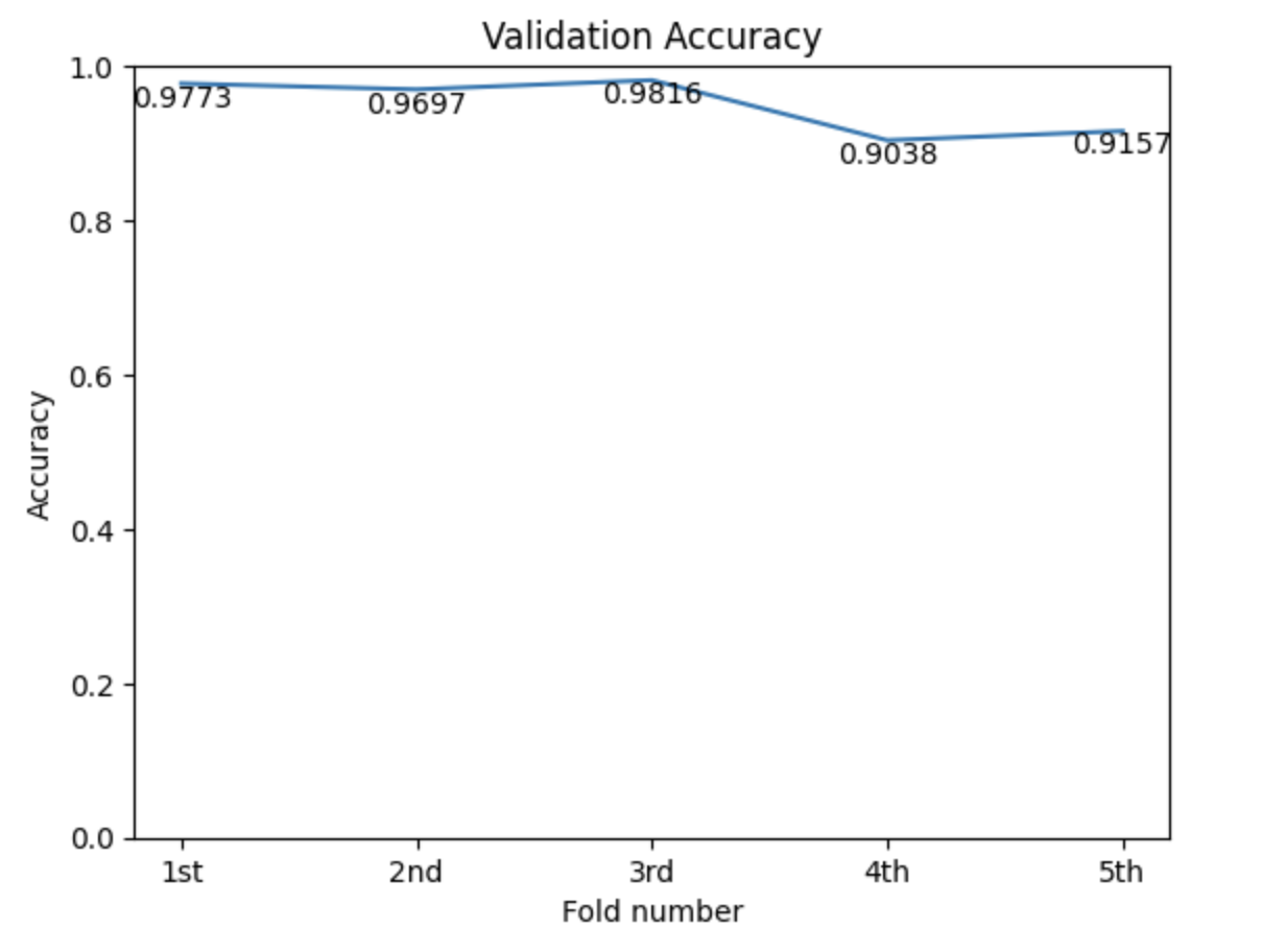
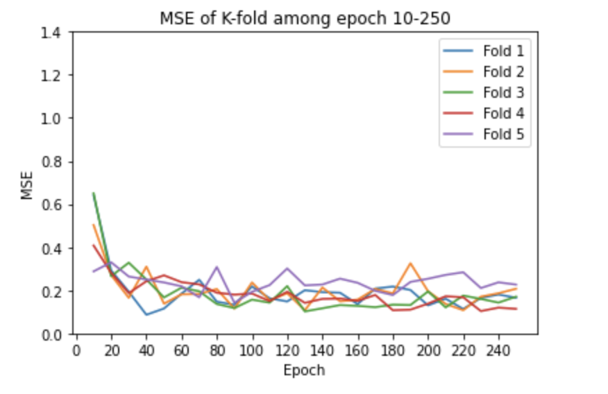
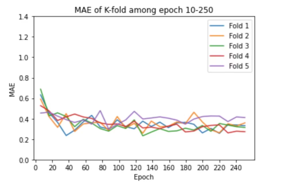
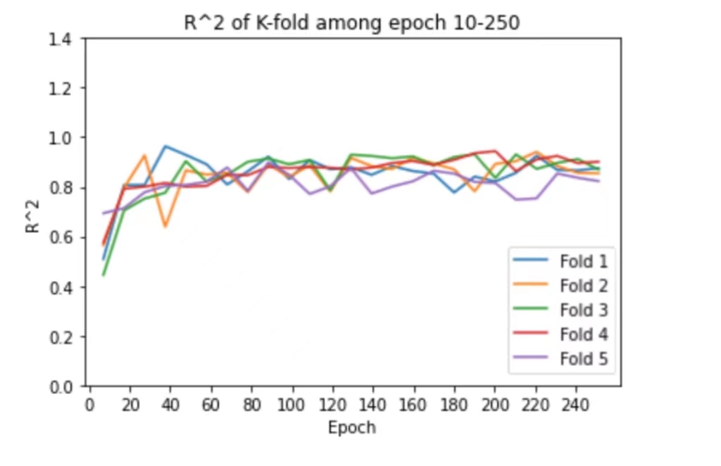
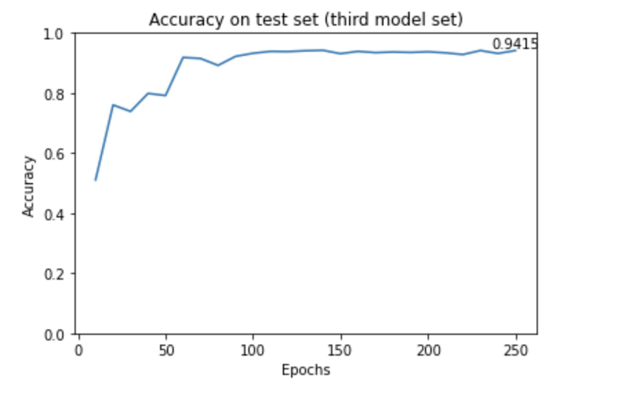
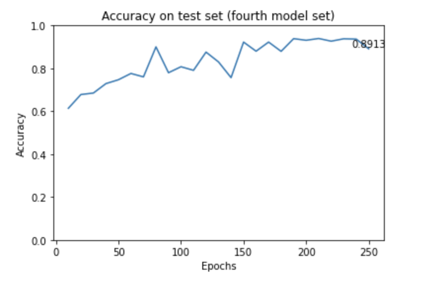
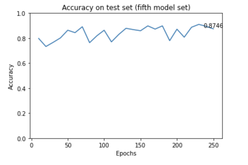
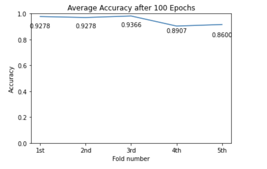
K-fold: In order to have a more accurate score, we used K-fold cross validation to train the model. We chose to use K = 5, which means we split the training dataset into 5 parts randomly, and each time we use 4 parts for training and 1 part for validating. We repeat this process 5 times and take the average score.

Algorithm

From a mathematical point of view, the point cloud data can be represented as a set of points in a vector space. The points can be denoted as a set:

\(P = \{ x_1,x_2,x_3,\dots ,x_n\} \in \mathbb{R}^N\), where \(x_i\) is a point in the vector space

Usually, we take N = 3, which represent the x, y, and z coordinates of the point but it can increase up to 6 which also contains the color.

The nature of a point cloud is that they are:

Unordered
Transformation invariant

this means the order of the points in the set and how the model is observed should not affect the final result as they are essentially the same teeth model.

To solve the first problem, we need to make the model independent from the order of input data. PointNet network uses a symmetric function to ensure the order is not changed. It uses a max pooling function to achieve this.

To solve the second problem, the PointNet network uses a transformation matrix, a T-net, to ensure the model is invariant to the transformation of the input data. The T-net is a 3*3 affine transformation matrix, and we apply this matrix to the input points.

                        
    class STN3d(nn.Module):
        def __init__(self):
            super(STN3d, self).__init__()
            self.conv1 = torch.nn.Conv1d(3, 64, 1)
            self.conv2 = torch.nn.Conv1d(64, 128, 1)
            self.conv3 = torch.nn.Conv1d(128, 1024, 1)
            self.fc1 = nn.Linear(1024, 512)
            self.fc2 = nn.Linear(512, 256)
            self.fc3 = nn.Linear(256, 9)

            self.relu = nn.ReLU()

            self.bn1 = nn.BatchNorm1d(64)
            self.bn2 = nn.BatchNorm1d(128)
            self.bn3 = nn.BatchNorm1d(1024)
            self.bn4 = nn.BatchNorm1d(512)
            self.bn5 = nn.BatchNorm1d(256)

Optimizer

We used Adam optimizer with a learning rate of 0.001. Adam is an optimization algorithm that can be used to update network weights with adaptive learning rates.

Loss function

We used the mean squared error as the loss function. It is a common loss function for regression tasks.

Classification -> Regression

We extended and implemented our model to fit our specific scenario. The original PointNet network is designed for classification tasks, but in order to make the network adapt to our requirements, we modified its structure to a regression neural network. We kept the two transformations and multi-layer perceptron layers to extract global features from the data, but we changed the last layer into a fully-connected layer with an output of one neuron. The structure of the model is shown in the figure below.

                                
# Regression 
class PointNetReg(nn.Module):
    def __init__(self, feature_transform=False):
        super(PointNetReg, self).__init__()
        self.feat = PointNetfeat(global_feat=True, feature_transform=feature_transform)
        self.fc1 = nn.Linear(1024, 512)
        self.fc2 = nn.Linear(512, 256)
        self.fc3 = nn.Linear(256, 1)
        self.dropout = nn.Dropout(p=0.3)
        self.bn1 = nn.BatchNorm1d(512)
        self.bn2 = nn.BatchNorm1d(256)
        self.relu = nn.ReLU()

    def forward(self, x):
        x, trans, trans_feat = self.feat.forward_1(x)
        x = F.relu(self.bn1(self.fc1(x)))
        x = F.relu(self.bn2(self.dropout(self.fc2(x))))
        x = self.fc3(x)
        return x, trans, trans_feat

Fig.3 - model summary

Experiments results & Evaluation

We evaluate our model in two ways: normal evaluation criteria for regression models and the accuracy after mapping the regression result to distinct tooth wear grades. We conducted detailed comparisons between different variants of the model.

Training and Validation

After data agumentation, we have 4626 point cloud models. As we used K-fold, where K = 5, we trained our model on 3700 point cloud models and validated it on the remaining models. In terms of the maximum number of epochs, we set it to 250 because the authors of the original PointNet paper used 250 which performes very well without overfitting. We also conducted an experiment to check if 250 epochs will cause overfitting on our training set.

Accuracy mapping: Only showing the predicted result (ie. decimal numbers) is not enough for dentists to evaluate patient tooth wear in practice. We therefore, decided to map the predicted result to actual tooth wear grades. We use the following mapping:

\(f: I \longmapsto N \)

\[ (- \infty, 1.5] \longmapsto 1, \\ \] \[ (1.5, 2.5] \longmapsto 2, \\ \] \[ (2.5, 3.5] \longmapsto 3, \\ \] \[ (3.5, \infty) \longmapsto 4 \]

While training, the first thing we want to ensure is the loss function keeps decreasing in the process and the accuracy is increasing.

Fig.4 - Training loss agianst epochs

Fig.5 - Accuracy against epochs

As we used K-fold, we trained our model 5 times on a random portion of the dataset (4/5) and the rest (1/5) would be used for validation. The following figure shows the loss and accuracy of the model on the validation set.

From the figure below, we can see that the mean squared error (MSE) on each validation set. The average MSE is 0.1371 and the average accuracy is 0.9496.

Fig.6 - MSE error on each validation across K-fold

Fig.7 - Accuracy on each validation across K-fold

Testing

After training the model, we evaluated their performance on the test set. The following figure shows how we use several evaluation metrics and accuracy to evaluate the models on the test set.

Mean squared error (MSE): is a commonly used metric to measure the difference between the predicted value and true values in a regression problem. For more details about MSE in PyTorch, please see here. The formula for MSE is:

\(MSE = \frac{1}{N}\sum_{i=1}^{N}(y_{pred,i}-y_{true,i})^2\)

The lower the MSE, the better the model is.

Here is the MSE of each trained model on the test set against epochs (10^th, 20^th, ..., 250^th).

Fig.8 - This line graph shows the MSE loss trend for different folds

Mean absolute error (MAE): is another commonly used metric. It is calculated by taking the average of the absolute differences between the predicted and true values. For more details about MAE in PyTorch, please see here. The formula for MAE is:

\(MAE = \frac{1}{N}\sum_{i=1}^{N}|y_{pred,i}-y_{true,i}|\)

Similar to MSE, we also want to minimize models' MAE error.

Here is the MAE of each trained model on the test set against epochs (10^th, 20^th, ..., 250^th).

Fig.9 - This line graph shows the MAE loss trend for different folds

R squared (coefficient of determination): shows how well the regression model explains observed data. The figure shows that the avarage R² is over 0.8 after 250 epochs of training.

Fig.10 - This line graph shows the R-squared loss trend for different folds

Accuracy: we use accuracy to evaluate the overall performance on the test set. After mapping the predicted result to tooth wear grades, we found that the average accuracy is 0.9140 after 250 epochs of training.