Algorithms - SightLinks

Algorithm Pipeline

Our comprehensive processing workflow from input image to georeferenced detections

Pipeline Overview

Our automated detection pipeline processes input imagery through six sequential stages to identify and localize target features with precision. The workflow begins with dynamic image segmentation, followed by deep learning-based classification to identify regions of interest within the image. These regions then undergo oriented bounding box (OBB) detection, with each identified crosswalk precisely georeferenced to real-world coordinates. The pipeline then intellligently filters the results, removing duplicate detections while maintaining accurate crossings. Finally, outputs are generated in multiple formats - simple text files for easy review and structured JSON for programmatic use. Complete technical specifications are provided in the following sections, with additional implementation details available on the dedicated implementation page.

1. Initial Segmentation

Since our models expect images of a certain size, we need to segment the images to those respective sizes. All image segmentation for both the classification model and bounding box model inputs are dynamic, this carries for all calculations which use the classification model input size and bounding box model input size.

The first stage divides the input images into sequential 256x256 pixel context windows. If a context window would extend beyond the original image boundaries, the system automatically shifts it inward to maintain the required size, while ensuring complete coverage of the source image. Each context window is uniquely identified with its row (y) and column (x) position, which corresponds to its relative location within the original image. This structured approach allows us to preserve the spatial relationships throughout the pipeline.

2. Binary Classification

In the second stage, each 256x256 pixel context window is evaluated by a classification model that returns a binary determination (True/False) based on whether its crosswalk detection confidence exceeds a given threshold. Context windows which return True are designated as "chunks of interest" with their row and column positions being recorded. If the row or column of interest is along the edges of the image, it is shifted by 1 row or column to the direction of the center (further explained in the filtering section).

For each context window of interest, the system dynamically re-segments the original image into a larger 1024×1024-pixel context window, centering the original 256×256 region to ensure full crosswalk containment and avoid truncation. If this expanded context window exceeds the image boundaries, it is adaptively shifted inward to maintain the required size.

The pipeline then generates geospatial metadata for the new 1024x1024 context window by deriving it from the original image's geo-referencing metadata. Each 1024x1024 context window is then stored along with its corresponding metadata, the original image's filename, and the row and column of interest which caused this context window to be created.

3. Bounding Box Detection

In the third stage of our pipeline, each 1024x1024 context window is processed through our oriented bounding box model to detect crosswalks, extracting both confidence scores and pixel coordinates for all four corners of each detected bounding box.

4. Georeferencing and Coordinate Transformation

The fourth stage of our pipeline handles the georeferencing of these corners using the context window's metadata. It converts these pixel coordinates into real-world locations, automatically interpreting British National Grid (BNG) for .jgw files or reading embedded spatial reference from GeoTIFFS.

These coordinates are then standardized to WGS84 (latitude/longitude) for consistency. Finally, the system stores each georeferenced detection in a dictionary—keyed by a combination of the original filename, and their row and column of interest—with values containing the WGS84-referenced boxes and their associated confidence levels.

5. Duplicate Filtering

The fifth stage of the pipeline now processes the georeferenced detections dictionary, using the known dimensions of both the initial classification context window and the bounding box context window. A critical overlap radius is calculated using the relationship between the bounding box context window size and the classification context window size (for more detail, check the implementation page). In our case, this leads to 5 rows and columns, which represents the maximum distance between rows or columns of interest where detections could share overlapping regions in the larger bounding box context windows. We will call detections which might overlap as "neighbors". This mathematical relationship explains the earlier edge-case handling (a row or column shift inwards if the row or column of interest is along the border), which serves the purpose of strategically minimizing the neighbor checking domain to those that could geometrically overlap without changing the bounding box (1024x1024) context windows generated.

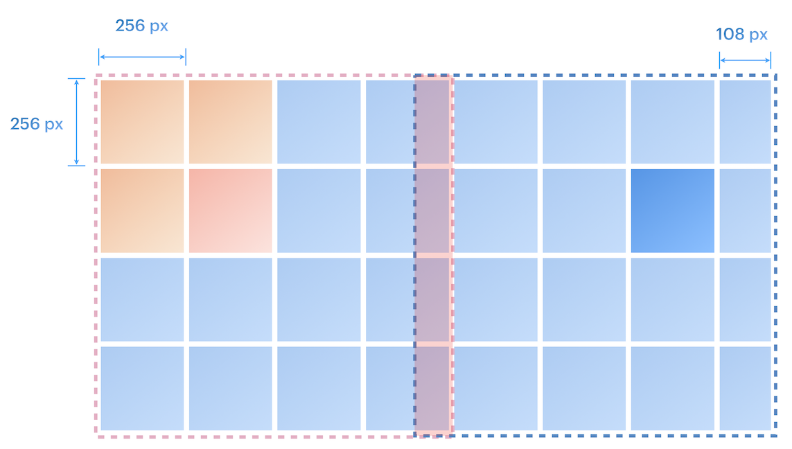
Visual representation of 1024x1024 context window overlap

From the visual representation, you can see that the orange and the red classification context window will generate the exact same larger red context window if they are a chunk of interest, and by shifting any of the orange box to the red box, it allows us to minimize the area checked for overlaps while keeping the same larger context window generated (for more detail, check the implementation page).

After defining the neighboring radius, the system processes each entry in the dictionary, checking for spatially adjacent context windows (neighbors) that may contain a duplicate. Using Non-Maximum Suppression (NMS), it compares all bounding box pairs between the current context window and its neighbors, discarding lower-confidence detection when their overlap exceeds a predefined threshold. Once all duplicates have been removed, the pipeline consolidates the remaining detections into a refined output dictionary, where each key corresponds to an original input filename, and its associated value contains all unique bounding boxes detected in that image, along with their confidence levels.

6. Final Output Generation

In the 6th stage of our pipeline, it creates our output. The pipeline saves the final detections dictionary contents to a JSON file, where each item stores the input image's base name, the oriented bounding boxes detected in the image (represented by a list of the four corners), and the confidence of each box.

Users can also choose to save it in a TXT file, where a TXT file is generated for each input file. The consolidated output provides a clean, filtered dataset of crosswalk detections ready for integration with mapping and navigation systems.

Data

This page covers the methodology used in our data collection, annotation and processing steps, for further information on alternative methods considered and a deeper reasoning for choosing each of these methods, please see our research section.

Dataset Overview

The dataset that we collected used satellite images from European pedestrian crossings, with a primary emphasis on satellite images on London and the surrounding regions. This geographical focus ensures high relevance for both urban and rural British environments, while still enabling compatibility for European urban environments. The downside to this is that deployment in other continents may require retraining with local data to compensate for different regional crossing standards.

Location Identification

The OpenStreetMap organisation has a comprehensive database of crossing locations in major urban cities in Europe, as well as an incomplete but sufficient database of crossing locations in rural areas. We generated and applied a standardised query for crossing locations within a square geolocational area to several major cities in the United Kingdom and Continental Europe, as well as rural towns in the Oxford region.

Region	No. of Crosswalks	Environment Type
London	8,912	Urban
Edinburgh	4,567	Urban
Glasgow	6,342	Urban
Oxfordshire	2,789	Rural
Barcelona	7,050	Urban
Paris	3,164	Urban

The data collection process focused on major urban centers and rural areas to ensure comprehensive coverage of different crossing styles and environments. London, being the primary focus, provided the largest dataset with over 8,000 crossings, offering diverse examples of urban crossing patterns. The inclusion of European cities like Barcelona and Paris helped validate the model's performance across different urban planning styles and crossing designs. The Oxfordshire region, representing rural environments, contributed valuable data on less dense crossing patterns and different road layouts. This geographical diversity ensures our model can handle various crossing configurations while maintaining high accuracy across different environments.

Image Acquisition

Crosswalks within a certain distance of one another were removed from the dataset to reduce repetitive data in the case of intersections and other dense traffic features that would cause overlapping image. For each crosswalk in the set, the associated satellite/aerial image was retrieved using the Google Static Tiles API. A consistent magnification level was used to standardize the resolution of the images retrieved. As a result of the limited precision of the location stored by OpenStreetMap's database, not all locations of crossings were centred in the image. Approximately 30,000 unique crossing instances were identified and retrieved.

Acquisition Process Steps:

Location Fetching:
- Retrieve crossing coordinates from OpenStreetMap's database over various geographical regions
- Filter out crossings that are too close to each other to avoid overlap
Satellite Image Retrieval:
- Use Google Static Tiles API to fetch satellite imagery
- Maintain consistent zoom level (level 20) for uniform resolution
- Retrieve images in 1024×1024 pixel dimensions
- Store images with unique identifiers matching crossing locations
Manual Labeling:
- Use YOLO-OBB visualization tools for annotation
- Mark four corner points of each crossing instance
- Store annotations in corresponding text files
- Include confidence scores for annotation quality

Annotation Methodology

Images were annotated manually using YOLO-OBB visualised labelling tools, according to a data annotation policy which ensured standardised quality and format of annotations. Annotations consisted of four pairs of (x, y) coordinates per crosswalks, defining an oriented bounding box, and were stored in a text file by the image that they were associated with. Geo-spatial coordinates were stored as reference material but were not used in the training process. A quality control process on the produced data using a visualisation tool discarded low quality annotations to ensure high quality data.

Dataset Composition

Total instances: ~30,000 (Estimated from labels.jpg visualisation)
Single class: "zebra_crossing"
Data format: Aerial imagery with world file (.jgw) georeferencing
Resolution: 1024×1024 pixel

Data Conversion Process

A slightly different methodology was used for generating the dataset used in the training of the classification layer. Three additional steps were added, as lower requirements for annotation quality allow augmenting the dataset using automated methods, to convert previous data collected into a compatible format and to adjust the data's distribution.

Dataset Augmentation:

All data queried for the classification dataset was done so at a lower resolution of 256×256 pixels. Labels were generated automatically according to the methods described below.

Additional positive label image data was acquired using a larger set of crosswalks retrieved from OpenStreetMap and the same Google Static Tiles API method
Additional negative label image data was acquired using an inverse method, where coordinates identified to not occur in the crosswalk dataset were used to retrieve images that did not contain crosswalks
Labels were stored in image, text-file pairs, where each text file contained a Boolean label for the associated image, represented by a binary value

Dataset Conversion:

The following was applied to each image in the previously discussed bounding box annotated dataset to convert it to a compatible format for classification training. Segmentation was applied to larger images to produce several 256×256 sub-sections of the image. Bounding boxes were generated corresponding to the sub-sections area in the original image, and an intersection-over-union (IoU) metric was calculated with each of the annotated bounding box labels.

Sub-sections that satisfied a threshold IoU metric with at least one labelled bounding box were given positive labels, while all other sub-sections were given negative labels.

The threshold is a hyper-parameter that has significant performance implications. Decreasing the threshold reduces the false-negative rate, as a lower portion of the crosswalk must be included in the image to be classified as including one. The inverse effect is true for the false-positive rate when increasing the threshold. To determine the threshold that would produce the model with the highest overall accuracy rate, several VGG classifier models were trained and used to evaluate a subset of unseen data with automated annotations. We chose a 30% threshold, which did not have the highest overall accuracy result, but had the lowest false positive before significant increase in false-negative rate as the threshold increases.

Selective Re-sampling:

The converted data from the manually annotated dataset has a higher reliability, as the automated labelling does not have human validation of occlusion over the crosswalks due to cars, trees or other obstructions. As such, the ratio of automated to converted data was maintained at a 1:1 ratio.

As a result, there were a skewed distribution of labels in favour of positive labels, at a 3:1 ratio. To reduce the false positive rate in the trained classifier due to potential over-fitting, resampling was applied to reduce the number of positive labels to a 2:1 ratio, to reduce the false positive rate.

Dataset Summary

Our dataset is extensive and, as of March 2025, is the largest open-source oriented bounding box annotated dataset of pedestrian crossings in satellite imagery. It is primarily focused on European crossings, with a particular emphasis on London and surrounding regions. This regional focus ensures high relevance for European urban environments but may require adaptation when applied to areas with different crossing styles or infrastructure designs. The dataset was built through a rigorous collection and annotation process, ensuring diverse representation of crossing types. However, users deploying the dataset in non-European contexts should account for potential variations in crossing layouts and urban planning standards.

Machine Learning Methodology

Methodology for localisation of crosswalks in satellite data

Classification Model (Initial Screening)

Architecture Evolution:

VGG16 (Initial Implementation) - 618MB
ResNet50 (Intermediate Implementation) - 98MB
MobileNetV3 (Current Implementation) - 21.8MB
Quantized MobileNetV3 - 2.8MB

Purpose & Features:

Binary classification of 256x256 image segments
Classes: Zebra crossing vs Background
Output: Binary prediction with confidence score
FLOPs count: 60 million (vs. 16 billion for intial VGG16 model)
Time per inference of 0.021 seconds (Nvidia 4070)

Crosswalks are generally spare features in satellite imagery, with most images lacking them. We leveraged this property to boost processing speed by implementing a lightweight classification model as an initial screening layer to filter out negative examples. Our classifier takes in small sub-sections of an input image and identifies the likelihood of a region of the image to contain a crosswalk.

Throughout development, we iteratively refined our model to optimize the efficiency-accuracy trade-off. Different model architectures were employed according to our changing requirements and an increasing need for speed, but eventually we chose MobileNetV3-small in the last two months of our project.

MobileNet has a distinct speed advantage over traditional machine learning models due to it using depth wise separable convolutions as a fundamental unit in its models. The traditional convolution operation is split into two parts: a depth wise convolution where filters are applied to each input channel on an individual basis, and a pointwise convolution where a 1x1 convolution operation is applied to combine the outputs of the depth wise convolutions. By factorizing this operation, the computation and model size required is significantly reduced.

MobileNetV3-small has a significant number of improvements compared to the original MobileNet architecture. Among these are the introduction of linear bottleneck, inverted residuals, squeeze-and-excite layers, and much more. These changes significantly improve performance over the original version.

Object Detection Model (Precise Localization)

Architecture & Variants:

YOLO 11 OBB (Oriented Bounding Box)
Available variants: nano, small, and medium
Default: nano (balanced speed/accuracy)
Precision gain from nano to medium: ~2.5%
FLOPs count: 17.2 billion (nano variant)

Pipeline Integration:

Used for precise crossing boundary detection
Output: 4-point coordinates defining crossing boundaries
Applied only to regions pre-filtered by classification model
Optimized for resource efficiency in large-scale processing

The core of our pipeline is the object detection layer, which leverages a YOLO-v11 model to process context windows and generate oriented bounding boxes corresponding to high confidence crosswalk predictions. Unlike traditional axis-aligned bounding boxes, our method captures objects with varying orientations, providing a more precise representation of spatial characteristics and significantly higher precision.

From the onset of our development, our chosen object detection model was YOLO-v11 (You Only Look Once). YOLO uses a convolutional neural network that processes the entire image input in one pass, rather than with separate identification and classification steps. As such, it has a significantly faster inference speed compared to similar models without compromising on accuracy or generalization.

YOLO typically outputs a set of bounding box coordinates with their associated class confidences, but our oriented variant has an additional rotation attribute θ. Although this is only a single addition, it causes significant issues with the generalized IoU loss functions used in training, requiring much more mathematically intricate and expensive loss functions. As a result, there is a significant increase in computational overhead, with YOLO-OBB v11-nano having 17.2 billion FLOPs as opposed to YOLO-v11-nano's 6.5 billion.

The precision improvement from the nano model to the medium model is around 2.5%, with accuracy increasing by about 3.0%. However, this comes with a significant computational cost, as the number of FLOPs increases by more than 10 times (from 17.2B to 183.5B). Despite this, we chose to default to the medium model for our deployed pipeline, as most of the processing is handled by the screening model, and we prioritize reliability over speed.

Model Architecture Details

Technical specifications of our deep learning models

MobileNetV3 Architecture Overview

Core Features:

Linear Bottlenecks: Preserves information flow in narrow network layers
Inverted Residuals: Expands features in intermediate layers for better representation
Squeeze-and-Excite: Adaptively recalibrates channel-wise feature responses
Hard Swish Activation: Computationally efficient non-linearity function

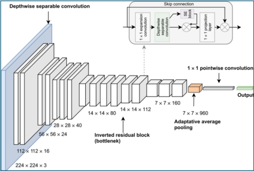
MobileNetV3 architecture with inverted residuals and linear bottlenecks

Performance Comparison:

Model	Size	FLOPs per Inference	Inference Time (s)
VGG16	618MB	16 billion	0.867
ResNet50	98MB	4.1 billion	0.3398
MobileNetV3	21.8MB	60 million	0.021
Quantized MobileNetV3	2.8MB	60 million	0.014

For the evaluation of our classification performance, we utilized a dataset consisting of 1,876 previously unseen classification images, with a distribution of 1,022 positively labeled images and 854 negatively labeled images. All evaluations were conducted on an NVIDIA 4070 GPU and repeated three times to account for any potential anomalies in inference time that could arise from background processes. The results were averaged to ensure accuracy.

YOLO-OBB Architecture

Oriented Bounding Box Details:

Rotation Parameter θ: Enables precise capture of non-axis-aligned objects
Custom Loss Function: Specialized function for oriented bounding box regression
4-Point Representation: Coordinates of all four corners for maximum precision
Rotated IoU Calculation: Accounts for orientation in overlap evaluation

YOLO-OBB architecture with oriented bounding box prediction

Variant Comparison:

Variant	FLOPs	Parameters	mAP50
YOLO-OBB 11 nano	17.2 billion	3.2 million	94.5%
YOLO-OBB 11 small	45.3 billion	11.1 million	96.2%
YOLO-OBB 11 medium	183.5 billion	25.9 million	97.0%
Standard YOLO v11 nano	6.5 billion	2.8 million	N/A (different task)

For the evaluation of our YOLO Rotated Object Detection model, we trained three models of varying sizes using the same training data and methodology outlined in our implementation. The models were then assessed based on their mAP50 score on a separate test set, consisting of 258 images containing a total of 744 crosswalk features.

Metrics Legend

Performance Metrics Explained

Precision: Precision measures the proportion of positive predictions that are actually correct.
Recall: Recall measures the proportion of actual positive instances correctly identified as positive.
mAP50: mAP50 (mean Average Precision at 50% IoU) is a performance metric for object detection models that measures how accurately objects are identified with bounding boxes. It calculates the average precision across all object classes, where a detection is considered correct if its Intersection over Union (IoU) with the ground truth is at least 50%.
mAP50-95: A more comprehensive metric for object detection, measuring the mean average precision across multiple IoU thresholds, starting at 50% and incrementing in intervals of 5% until 95%.

YOLO Training Report Metrics

Box Loss

Initial value (Pre-trained): 2.31
Final value (Fine-Tuned): 0.61
Significant reduction in localization error throughout the training process.

Classification Loss

Initial (Pre-trained): 3.56
Final (Fine-tuned): 0.40
Strong improvement in classification accuracy as the fine-tuning

DFL Loss

Initial (Pre-trained): 2.03
Final (Fine-tuned): 1.12
Balanced feature learning

Visualization Metrics

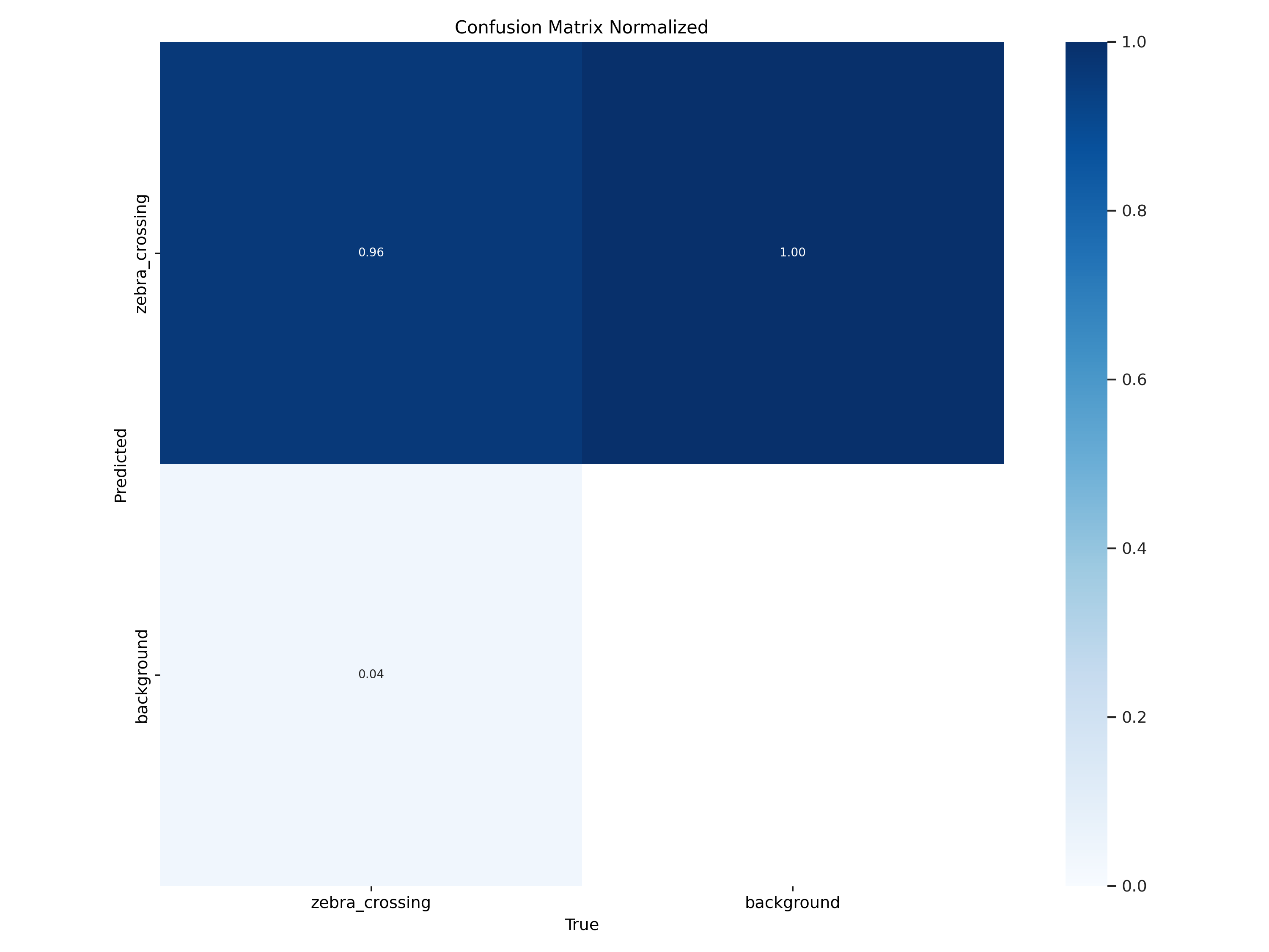
Normalised Confusion Matrix of YOLO V11 Medium's predictions, displaying the difference between predicted and ground truth bounding boxes during validation.

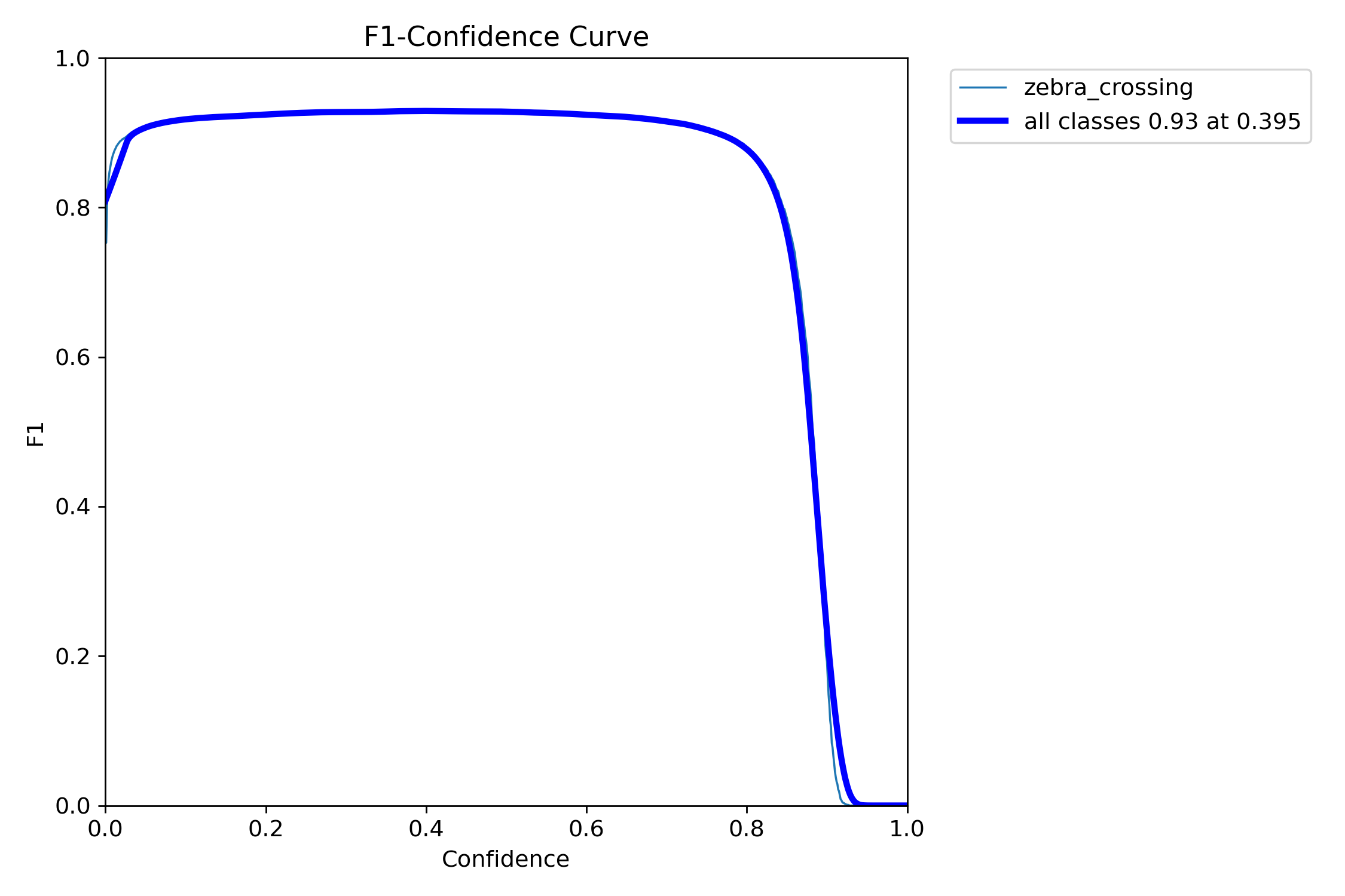
F1-Confidence trade off curve for YOLO V11 Medium, displaying how the F1 metric changes as we adjust the confidence threshold hyperparameter.

False Positive/Negative Rate curve showing the relationship between detection confidence threshold and error rates.

Hyperparameter Optimization

We conducted fine-tuning of the two primary hyperparameters in our system: the confidence threshold required to consider a prediction successful for each AI layer. Using our evaluatory framework, we incrementally adjusted these thresholds to optimize performance.

For the classification layer, we analyzed the false positive and false negative rates as the confidence threshold increased, while for the image detection layer, we evaluated performance using the F1 metric as the confidence interval increased.

By maximizing overall accuracy and F1 score, we determined that the optimal classification threshold is 0.35 to minimize false positives, while the object detection threshold is set at 0.5.

Discussions of Methodology

Understanding current constraints and pathways for future improvements

Potential Causes of Failure

The primary bottleneck in our current pipeline stems from model performance limitations, while other algorithmic components function as intended. Both our classification and OBB detection models exhibit reduced reliability when processing suboptimal satellite imagery - particularly under challenging lighting conditions, with obscured or faded crossings, or in low-resolution scenarios. The classification model's initial filtering sometimes incorrectly rejects valid crossing segments, while the YOLO-based detection system demonstrates dual failure modes: missing genuine crosswalks (false negatives) and misidentifying similar-looking features as crossings (false positives).

We attribute these shortcomings primarily to training data deficiencies, including insufficient sample volume and imperfect annotations where some crosswalks were completely unlabeled in the training set. These data quality issues likely explain the model's tendency to both overlook genuine positives and generate false detections on visually similar patterns.

Improvement Suggestions

To enhance our system's performance, it is essential to begin by improving the quality of our training data. Ideally, the dataset should encompass a wide range of environmental conditions—such as varying lighting, weather, and resolutions—while maintaining precise annotations to reduce labeling errors. Additionally, employing data augmentation techniques like adding synthetic noise, introducing occlusions, and applying perspective distortions can help the model become more robust to real-world imperfections.

After addressing data quality, upgrading to a more accurate model architecture may significantly boost detection reliability. Our current YOLO-based setup was chosen for its lightweight design, which is critical given our limited GPU resources. However, future deployments may benefit from using Rotated Faster R-CNN, which provides higher accuracy for oriented object detection—albeit with slower inference speeds. This trade-off between speed and precision should be evaluated according to the specific requirements of each deployment. If achieving higher confidence in detection is paramount, transitioning to a more advanced model may be justified despite longer processing times.

Experimental Results