Algorithms

Table of Contents

1. Description of Algorithms
2. Experiment setting
3. Experiment results and Discussions
1. NLP Processors
2. 5-Class Star Rating
3. Helpfulness
4. Conclusion
5. Reference

Top

Description of Algorithms

We’ve experimented with a large number of Natural Language Processing (NLP) and Machine Learning (ML) algorithms to achieve our goal, which is to predict a review’s staring and helpfulness from its text. The NLP algorithms we’ve used include Bag Of Words (Unigram), N-grams (CountVectorizer), Term Frequency-Inverse Document Frequency (TF-IDFVectorizer) and Word Embedding. The ML algorithms include Linear Regression, Logistic Regression, Decision Tree, Random Forest, Gradient Boosting Machine, Feedforward Neural Network and Convolutional Neural Network.

Here, we’ll explain the theories behind some of the complex algorithms, whilst the descriptions of the simple ones can be found under Research page.

Linear Regression

The most basic machine learning would be linear regression. It is a model that assumes a linear relationship between variables (x) and value (f(x)). For models with one variable only, it is as simple as solving the equation f(x) = m * x + c, finding the value of m and c and using them to predict f(x) for some x that’s unknown.[2] However, things can be more complicated with multiple variables,e.g., for our project, the variables are a list of numbers that represent the occurrence of different words/n-grams. That’s when techniques like cost function and gradient descent come into place.

The idea of the cost function is that: since the actual data won’t always fit into a perfect line (even if they have a very strong linear relationship), our goal is to find a hypothesis function h(x), which predicts the value from x as accurate as possible. And the accuracy is measured by the cost function. It simply calculates the average difference between the actual value and the value predicted by h(x). If we can find an h(x) with minimal cost, that h(x) would be the most accurate model.[3]

In order to reduce the cost, gradient descent is used. It first selects a point on the cost function graph and uses differentiation to find the direction towards the local minimum point. It then changes the constants of h(x) (which are the variables in cost function) bit by bit, so the function gradually approaches the local minimal point (and for linear function local minimum is same as the global minimum). Once it reaches minimal, the variable values of cost function will be used as constants in h(x), and a hypothesis with good accuracy is produced.[4]

Logistic Regression

Although linear regression is great, it’s not ideal for classification problem, because its range is ±infinity since it’s a y = mx + c type of function, which is not desirable as we want to yield probabilities of object x belonging to a certain class, which should always be between 0 and 1. As such for our first model we decided to use logistic regression which remedies this problem. Logistic regression always outputs values between 0 and 1. This is because its hypothesis function uses a logistic function f(t) = 1 / (1 + e-t) where t is usually the output from what would’ve been the hypothesis function in linear regression. [5] In fact, logistic regression works quite similarly to linear regression.

The cost function is also adapted using logarithms and when during training the hypothesis function’s prediction is compared to the real value y, the cost approaches infinity as the difference between h(x) and y approaches 1. In other words the more the hypothesis is incorrect, the more severe the punishment (and rate of change of punishment increases drastically). [3]

Decision Tree and Random Forest

As introduced in Research section, Decision Tree typically uses Gini Impurity to measure the quality of a split and find out what’s the best parameter to use in next node. Gini Impurity is calculated through:

Where Pi means the probability of choosing the i-ith item.

I.e., it picks a random sample from the set, and picks a random label based on the proportions of labels in this set, and measures the possibility that this sample doesn’t match the label.[6]

As for the Random Forest, It simples splits the whole data set into sub data sets and trains Decision Trees with them. When predicting for an unseen sample, it simply feeds the sample to all the trees and asks them to vote for a final answer.

Gradient Boosting Machine (GBM)

A GBM mainly contains three components: a cost function that needs to be optimized, a large number of weak learners and a method of combining results of weak learners into the cost function. In our case, the cost function will be logistic function and weak learners are Decision Trees. [10]

The GBM first fits itself to the training data and gets a cost function. It will also produce some values for parameters that are not optimal. Then it fits many small Decision Tree Regressors using not the original train data but the costs. By adding the values predicted by Decision Trees to the parameter values, the overall cost can be further optimized. [11]

Feedforward Neural Network

Feedforward is the most basic Neural Network (NN). As its name suggests, data will be passed forward through the NN and not feedbacks are provided between layers. [7] During training, NN passes train data through all the layers and generates an output through equation: o = g(w * x + b), where g() is the activation function (relu, sigmoid etc), w and x are weights and inputs from previous neurons and b is a constant used as bias term.

After the neurons in the output layer have produced their results, NN then calculates the loss between the predicted value and actual value and uses gradient descent to adjust the weights according to the loss. This is done backwards, i.e., weights of neurons in the last layer will be adjusted first. The maths equation would be:

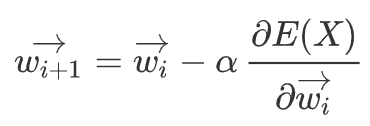
where Wi+1 means next weight, alpha is learning rate and E(X) would be the loss (e.g., mean squared error for regression problem). Thus, it is able to “learn” from the sample and will do better next time it performances a similar task. [8]

Convolutional Neural Network

Convolutional Neural Network (CNN) is generally considered to be better than regular feedforward NN in the area of image recognition and NLP. It is able to capture the information related to positions of pixels or sequence of words, which can be very helpful for the model to actually “understand” the inputs.

It works by having one or more Convolutional layers first, usually followed by a Max Pool layer, then the regular hidden and output layers. A convolutional layer is able to apply filters to the input and calculates the output based on values that are filtered. E.g., applying a filter of size 2 to input (1,2,3,4) will produce an output of (a,b,c,d), where “a” is calculated from (1,2), “b” is calculated from (2,3), “c” is calculated from (3,4) and the final “d” is the bias term. Max Pool layer is then used to reduce the complexity of the output and potentially prevent overfitting. It does this by only taking the maximum value among filter values. E.g., applying Max Pool of size 2 converts (a,b,c,d) to (max(a,b),max(c,d)). [9]

Experiment setting

Data Source

The data we used in this project comes from our client - Ocado’s website. It is a single CSV file containing information about 444,340 reviews. The information includes review time, an integer for product ID, an 0 or 1 integer indicating whether the reviewer has recommended this product to other customers, review title, review text, an integer in range 1 to 5 indicating the star rating, an float number indicating the helpfulness of this review and an integer indicating the number of people who rated its helpfulness.

Among those data, we used review title, review text, star rating for star rating prediction and review title, review text, star rating, helpfulness, vote counts for helpfulness prediction. (star rating was used in helpfulness prediction because we found a certain relationship between it and helpfulness during our experiments).

Training and Testing Set

To ensure the fairness in our experiments, we’ve split the original dataset into two files: one containing 434,340 reviews used for training and validation, another containing the rest 10,000 reviews used only for testing in the final comparison among models to obtain a fair and accurate score.

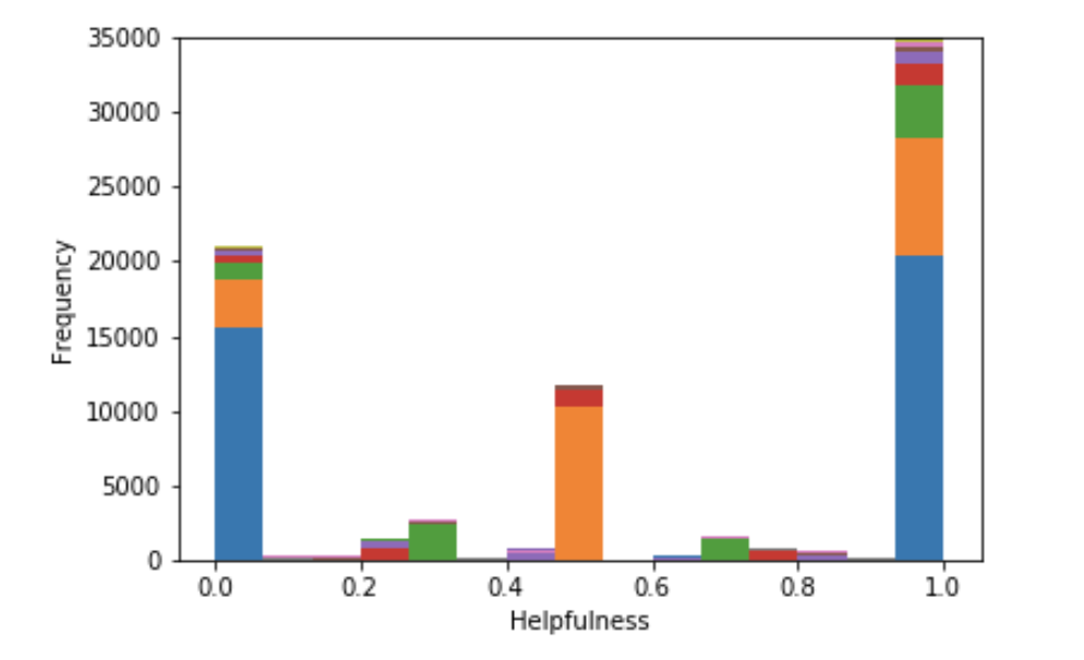
During the actual training, we’ve managed to filter many “bad samples”. In terms of star rating, we discovered that models trained with a balanced dataset (i.e., the numbers of reviews in each category are the same) would have better performance. Thus we used undersampling to filter out redundant reviews and got a dataset with 167535 reviews. As for helpfulness, we simply removed reviews that don’t have any votes -- otherwise, they’ll show as 0% helpful and significantly affect the model’s ability to learn from data.

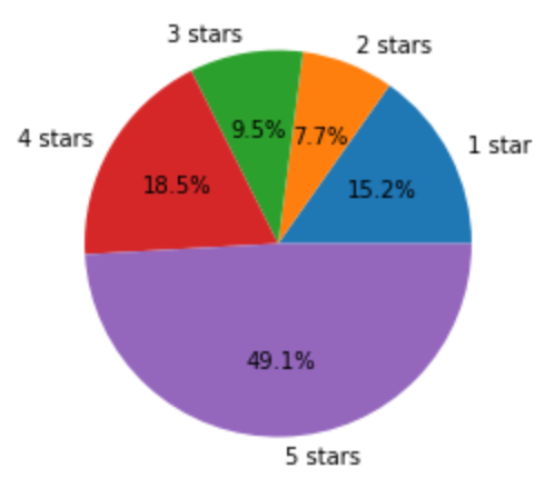
[Distribution of reviews with different stars in original dataset]

In practical, although we would love to make use of all the data, concerning the hardware limitations and time efficiency, we decided to only use 100k data to train and 5k data to validate.

Training and Testing Scheme

In order to obtain accurate scores, we’ve applied the technique of K-Fold Cross-Validation. It works by splitting the dataset into k subsets, using k-1 of them to train the model and the remaining one to validate the model. When experimenting with Cross-Validation, we fixed at 100k data with 5 folds, i.e., 80k training data and 20k validating data.

Cross-Validation is great, but it comes with a lot of issues in practice:

1. It takes longer to compute. With k folds, the same model will be trained and tested k times.
2. Sometimes it’s simply not applicable. E.g., when doing star rating predictions, we require the model to be trained with balanced data but still validated and tested against original data. In such cases where training and testing data come from two different datasets, doing a Cross-Validation is impossible.
3. Lack of support to additional hyperparameters. E.g., we used vote counts as sample weights to train the helpfulness prediction model, as this way we can reduce the influence of inaccurate samples. However, Scikit-learn, which is the ML training and evaluation library we used in this project, has not supported sample weights for Cross-Validation yet.

Due to the above aspects, in our later experiments, we tend to select 100k training data and 5k validation data randomly from the overall dataset. But of course, this was carefully done to make sure two datasets never overlap with each other.

We then used the separate test data file that contains 10k reviews that have never been used before to do the final evaluations. Thus, our models were not tuned for a certain set of data and should have a stable performance on any unseen data.

As for the methods of measuring a model’s performance, we used Mean Absolute Error to evaluate helpfulness models, as they’re regressors. The lower the error the better the model. In terms of star rating prediction, we used accuracy to measure the performance in the first place, but we soon realized that accuracy is not ideal, especially when the dataset is not balanced -- for instance, when 50% of the reviews are 5-star reviews, a model can easily achieve 50% accuracy by assuming all the inputs are 5-star reviews. It, however, is obviously a poor model when it comes to actual performance. In contrast, we used a better measurement called F1 Macro score.

F1 works by calculating a model’s precision (out of all samples it classified as class A, how many of them are correct) and recall (out of all samples that actually belong to class A, how many are classified to A correctly). It then combines them by the equation: f1 = 2*((precision*recall)/(precision+recall)), which becomes very small once any of the two numbers is small. Macro means F1 scores for all classes are equally weighted.[1] With this method, we can measure our models’ performances more accurately. The higher the F1 Macro score, the better the model.

Experiment results and Discussions

We’ve carried out a large number of experiments. Here, we’ll only discuss the crucial ones that have affected our decision of the final model. Details of the rest of experiments can be found in “jupyter” fold in our source code submission.

NLP Processors

Bag of Words/Ngrams

At first, we decided to use bag of words. However, bag of words model can be unreliable as it doesn't take any account of the context the word is used in. Common phrases like "out of date" "not very good" "not great" should have a very negative weight. In the current bag of words model words like "good" "great" "nice" have low weight, as they are used in both positive and negative review. So, we decided to use bag of ngrams. This model is going to give ngrams like "is good" a high positive weight and ngrams like "not good" a high negative weight.

Accuracy of bag of words and logistic regression model:

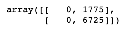
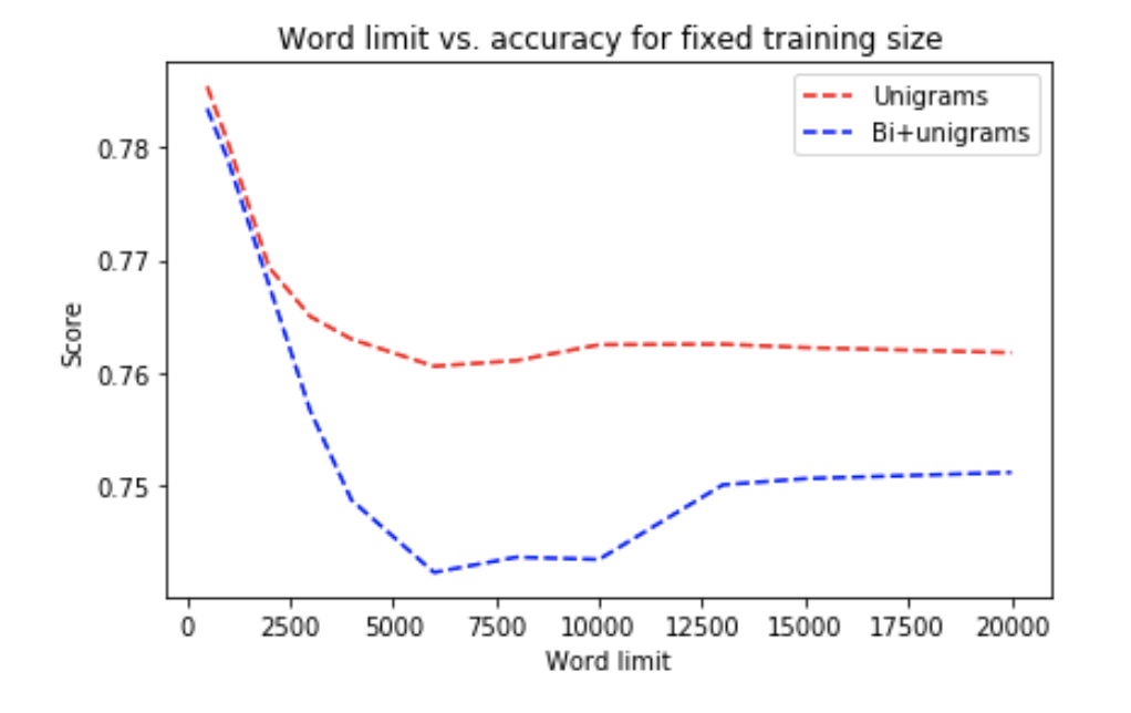
Accuracy of unigrams + bigrams and logistic regression model:

This shows that using bag of ngrams perform significantly better than using bag of words. Essentially, uni+bigrams with 5k vocabulary limit seems to achieve a good balanced between performance and efficiency, thus we decided to use this in our future experiments.

CountVectorizer/TfidfVectorizer

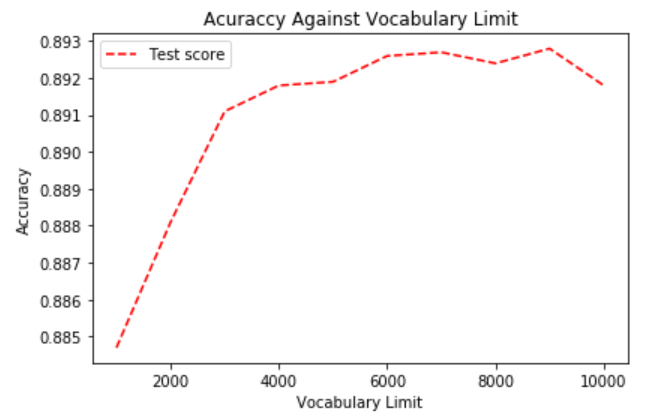
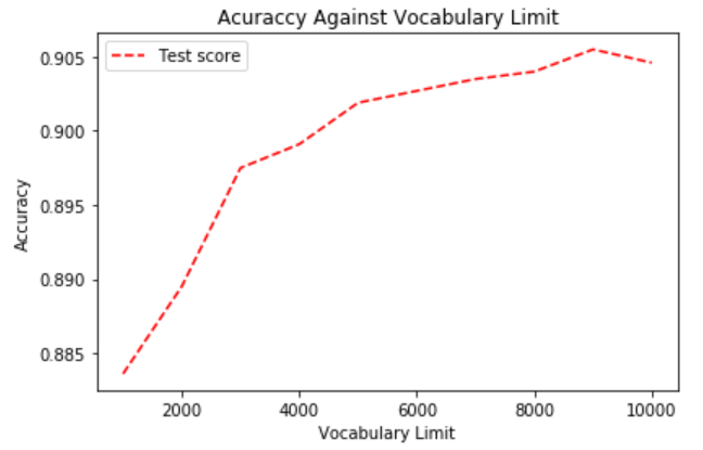
We Also compared the performance difference between CountVectorizer and TfidfVectorizer for different models. Tfidf means term frequency times inverse document frequency. In a large text corpus, words like “the”, “a”, “is” will appear very often and hence carrying very little meaningful information about the actual contents of the document. inverse document frequency diminishes the weight of terms that occur very frequently in the document set and increases the weight of terms that occur rarely. The performance difference between the two vectorizers depends on the machine learning model used and what are we trying to predict.

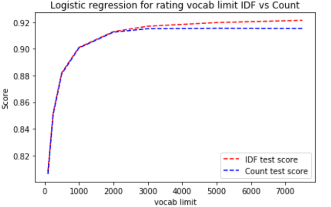
For logistic regression on rating. It seems that for TfidfVectorizerthe the more the vocab limit the higher the accuracy. For the CountVectorizer, the optimum accuracy is archieved when vocab limit is 3000, the accuracy decrease as vocab limit increase.

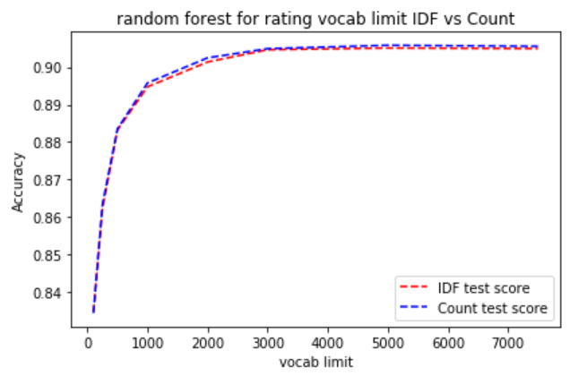
This is the comparison between CountVectorizer and TfidfVectorizer for random forest model on binary classification of positive and negative review. It shows that both vectorizer have similar performance.

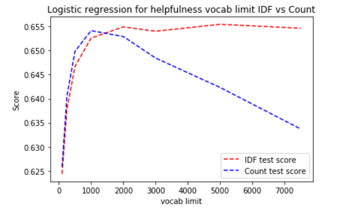
This is for logistic regression on helpfulness. For the Tfidf vectorizer, it seems that the more the vocab limit the higher the accuracy. For the CountVectorizer, the optimum accuracy is archieved when vocab limit is 500, the accuracy decrease as vocab limit increase.

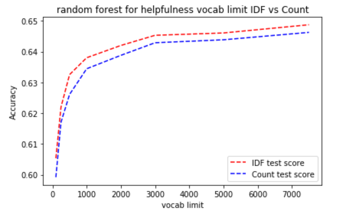
This is the comparison between CountVectorizer and TfidfVectorizer for random forest model on helpfulness. For both Vectorizer, the accuracy increases as the vocab limit increases. Tfidf seems to perform slightly better.

5-Class Star Rating

Logistic Regression

1. Penalty Scheme

There are two penalty schemes available for Logistic Regression: L1 (least absolute deviations) and L2 (least squares error). At that stage, we’ve yet developed experiments with balanced training set, thus we trained and validated data using 5 fold Cross-Validation. The result is shown below.

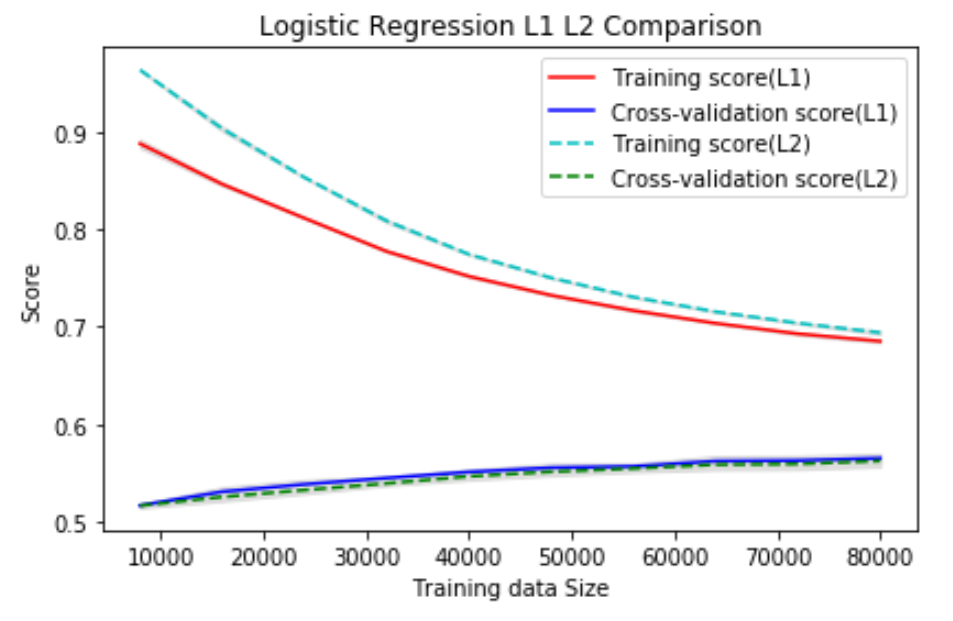
No obvious difference is observed. Since L2 is considered more stable (i.e., small changes in samples won’t cause the final model to be very different), it is the preferable choice.

2. Multiclass Schemes and Solvers

For Multiclass Logistic Regression, additional parameter “multi_class” needs to be specified. It controls how the model will put samples into multiple classes. If it is set to “ovr” (One versus rest), it will try to do a binary classification for each label. If it is set to “multinomial”, it will minimize the overall cost and solve all the problems together. In addition, Scikit-learn has different solvers and they each support different penalty schemes or multiclass schemes. However, we don’t expect them to affect the model’s performance. We compared those two schemes using the same testing scheme mentioned above.

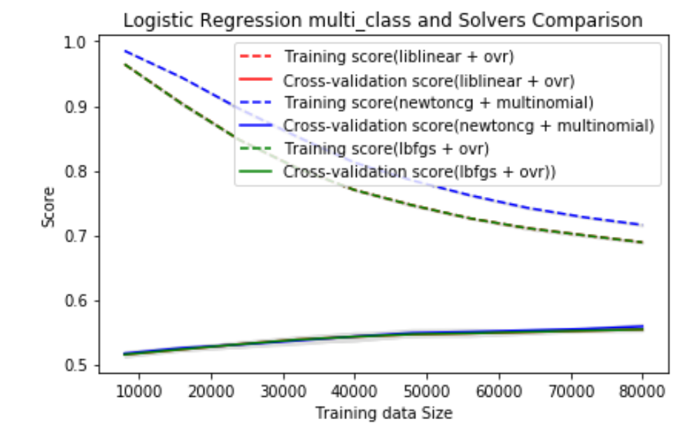
As expected, using different solvers doesn’t make any difference to score (red lines are not visible here because they perfectly overlap with green lines). Besides, We can't really see any difference in "ovr" and "multinomial". This makes sense because essentially they're just different ways of doing Logistic Regression. Since "ovr" is similar to binary Logistic Regression model we've experimented before, and it suffers slightly less from overfitting (as training scores are lower), we decided to use "ovr" instead of "multinomial".

3. Regularization C

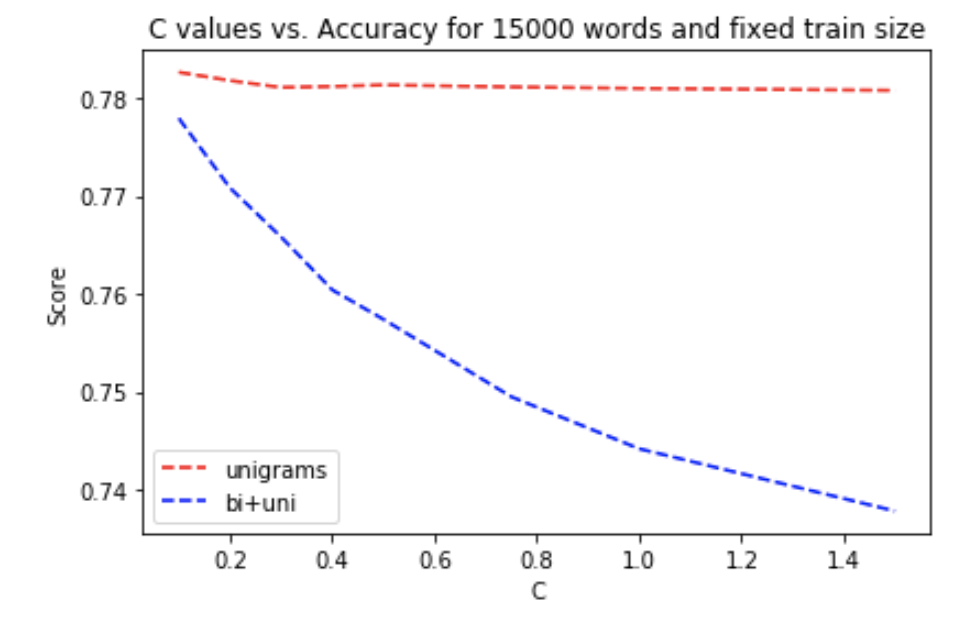
The regularization strength in Logistic Regression is controlled by hyperparameter C, which should be a float within range 0 and 1. Smaller the value indicates stronger regularization.

Initially, we used the same testing scheme (100k unbalanced data 5 fold Cross-Validation) and got the following result:

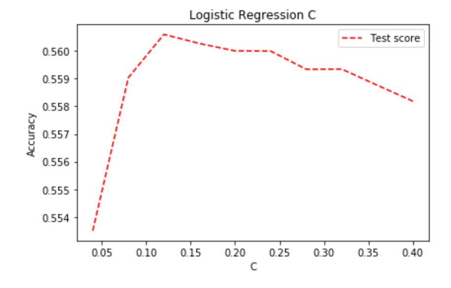
So a C value of 0.12 would give the best model.

However, later experiments suggested that C=0.12 is not optimal when trained with the balanced dataset. Thus, the same tests need to be carried out again on the balanced dataset. Here we used 100k randomly chosen balanced data to train and 5k randomly chosen unbalanced data to validate. Cross-Validation is not applicable, thus the score is less smooth.

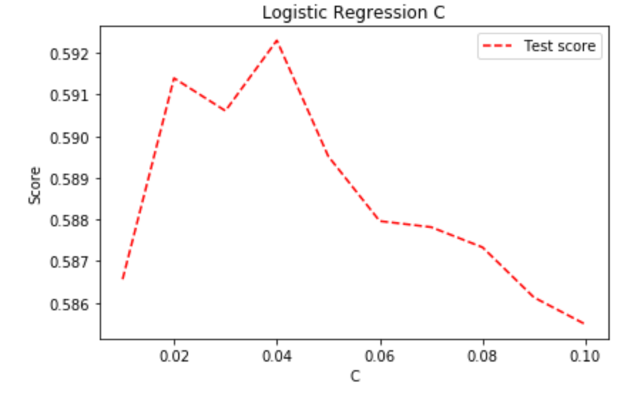
Now the optimal value for C is 0.04. We believe the reason why C should be set to a smaller value (i.e., stronger regularization) when using balanced dataset is that balanced dataset contains more noises. In the original dataset, most of the reviews are 1-star or 5-star, thus the features passed to Logistic Regression should mostly be extreme words, such as "Great", "Delicious", "Worst". When using balanced dataset, the model is forced to take the same amount of reviews from different classes, so it's not rare to have many neural words that don't help a lot in distinguishing the star rating.

4. Confusion Matrix

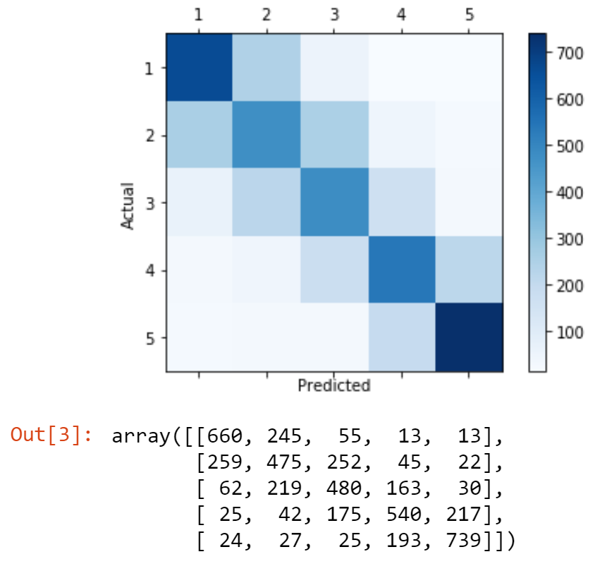
In the end, it would be interesting to plot the model’s Confusion Matrix to see its performance on different reviews.

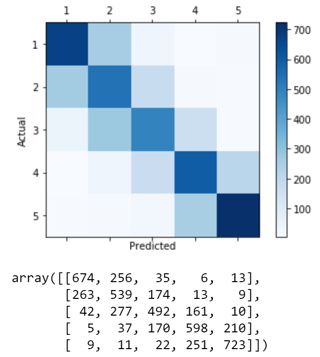
To allow a clear and straightforward view, all Confusion Matrices are plotted using 5k balanced dataset.

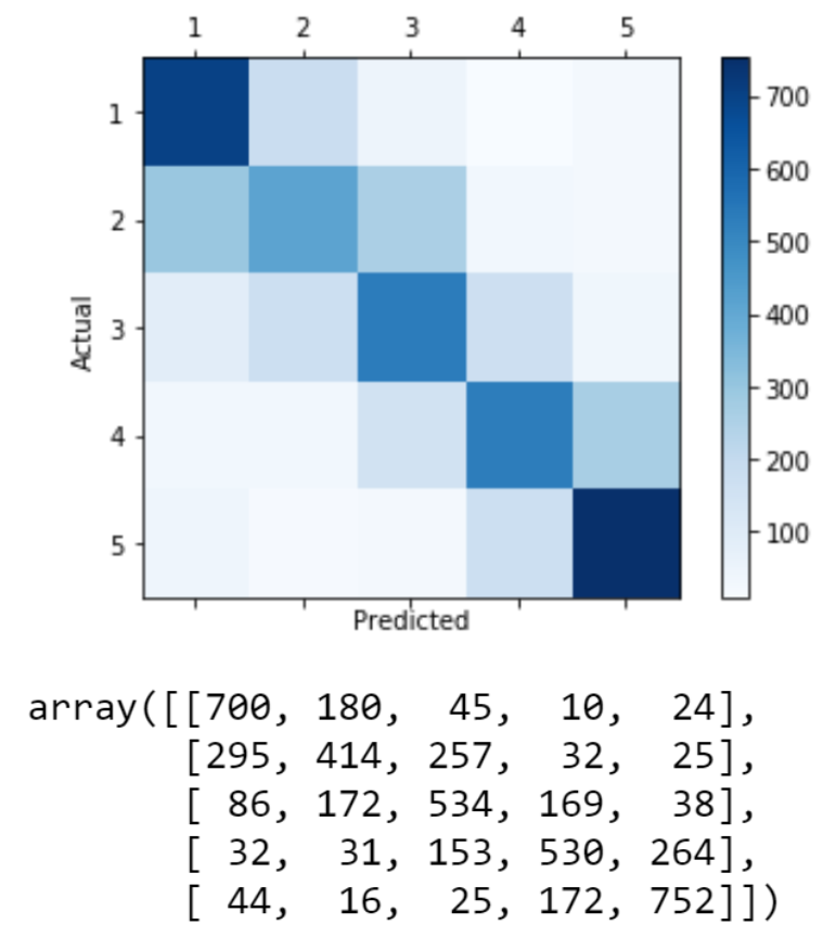
We see our model is good at predicting 1-star and 5-star reviews, but not that good when facing 2-star to 4-star reviews. Apart from that, it shows a regular pattern -- the further away the predicted class is from actual class, the fewer samples are included, except for 1-star and 5-star reviews where quite a few reviews are predicted to completely opposite sides. After some extra experiments, we found out those are typically reviews that compare a product to a different product, thus the text would contain many opposite words used to describe another product, and our uni+bigram NLP processors is not able to capture that.

5. Conclusion

To conclude, the best hyperparameters for Logistic Regression are: “l2” penalty, multi_class="ovr",C=0.04.

Random Forest

Before going into Random Forest, we did some experiments with Decision Tree on a simplified star rating problem. Since that’s only to improve our understanding and results are not used to decide the final model, they are not included in this report.

1. N Estimators / Number of Decision Trees

As Random Forest is a very robust method, it usually doesn’t suffer from overfitting at all, meaning more estimators will always give a better score. However, considering the time efficiency, we still need to find a value that balances the running time and model performance.

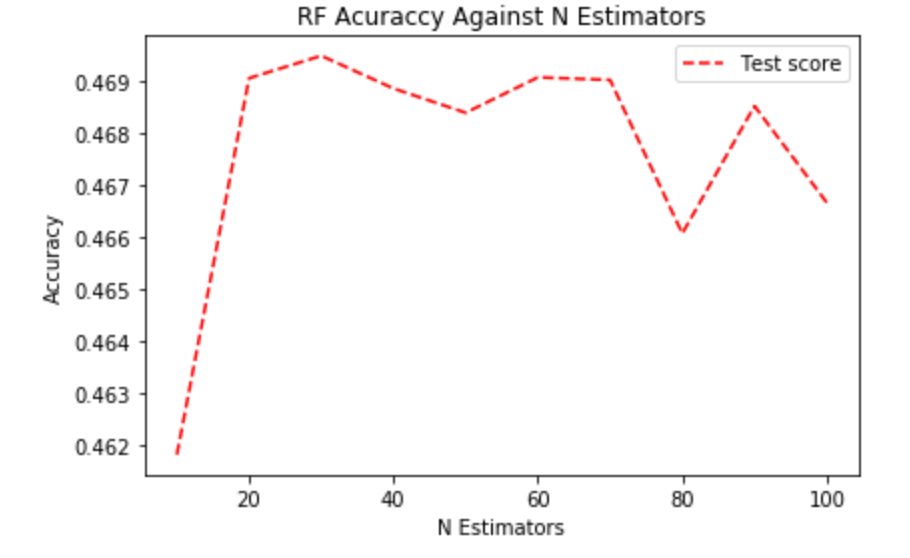
First, we tested it with unbalanced data and found out only 20 estimators are needed.

Then we experimented it with balanced training data:

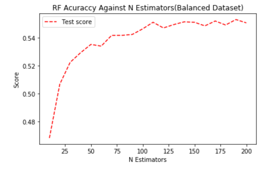
This time we see the score constantly improves till 200, but the rate of increase is not significant after n_estimators=100. We believe the reason why more estimators are needed when using balanced dataset is because of Decision Tree’s splitting scheme. Here we used a scheme called Gini Impurity, which is greatly affected by the distribution of training dataset. When training dataset is balanced, it would suggest the Decision Tree to split based on keywords that distinguish less common reviews apart (e.g., 2-star and 4-star reviews) instead of just focusing on the extreme words (e.g., “great”, “good”, “bad”). Hence, Random Forest is able to learn more from the data and more estimators should be used.

To reach a good balance between running time and performance, we decided to use 100 Decisions Trees.

2. Balanced Training Data

After the above experiments, we have enough data and knowledge to experiment with balanced training data. We trained Logistic Regression and Random Forest with 100k balanced and imbalanced data, then calculated their F1 Macro score using 5k imbalanced data.

Using balanced dataset to train models can greatly enhance their performances.

We believe it is because, with balanced training samples, more 2-star and 4-star reviews will be included. Thus the model won't focus heavily on 1-star and 5-star reviews only and is able to classify uncommon reviews correctly, hence the F1 Macro score is increased.

After this experiment, we went back to important tests we’ve done before and repeated them on the balanced dataset to ensure the results are the same.

3. Confusion Matrix

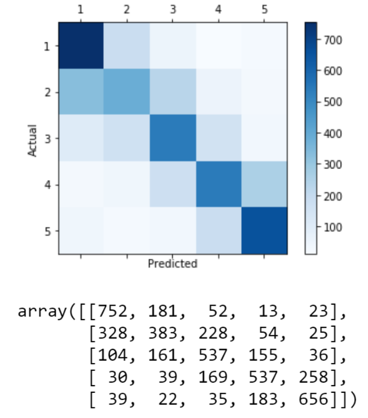
The matrix is very similar to the one from Logistic Regression.

4. Conclusion

The best hyperparameters for Random Forest are: n_estimatros=100

Gradient Boosting Machine (GBM)

Since GBM is heavily based on Logistic Regression, we used our previous experiments with NLP on Logistic Regression to assume that uni+bigram TF-IDF with 5k vocabulary limit works best for this model.

In addition, experiments carried out with GBM all used 5 fold Cross-Validation on 100k balanced dataset. Due to F1 Macro score’s nature of ignoring the distribution of test dataset, scores obtained in these experiments will only be slightly different from scores obtained by using an imbalanced test set (less than 0.01). Other experiments also suggested that the plots are identical, i.e., the optimal hyperparameters are the same. This decision is made because of the difficulty in evaluating GBM’s performance -- without Cross-Validation, scores tend to fluctuate a lot and make it very hard to tell which one is the highest.

1. N Estimators

Similar to Random Forest, we investigated how many “weak learners” will cause GBM to overfit.

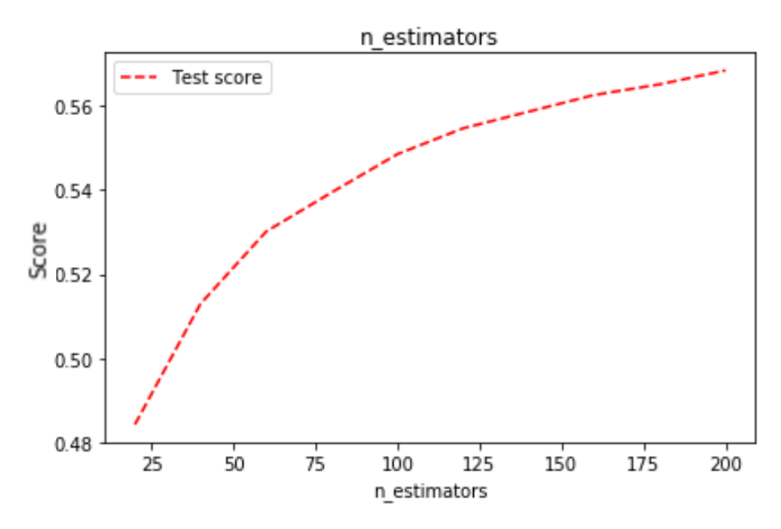
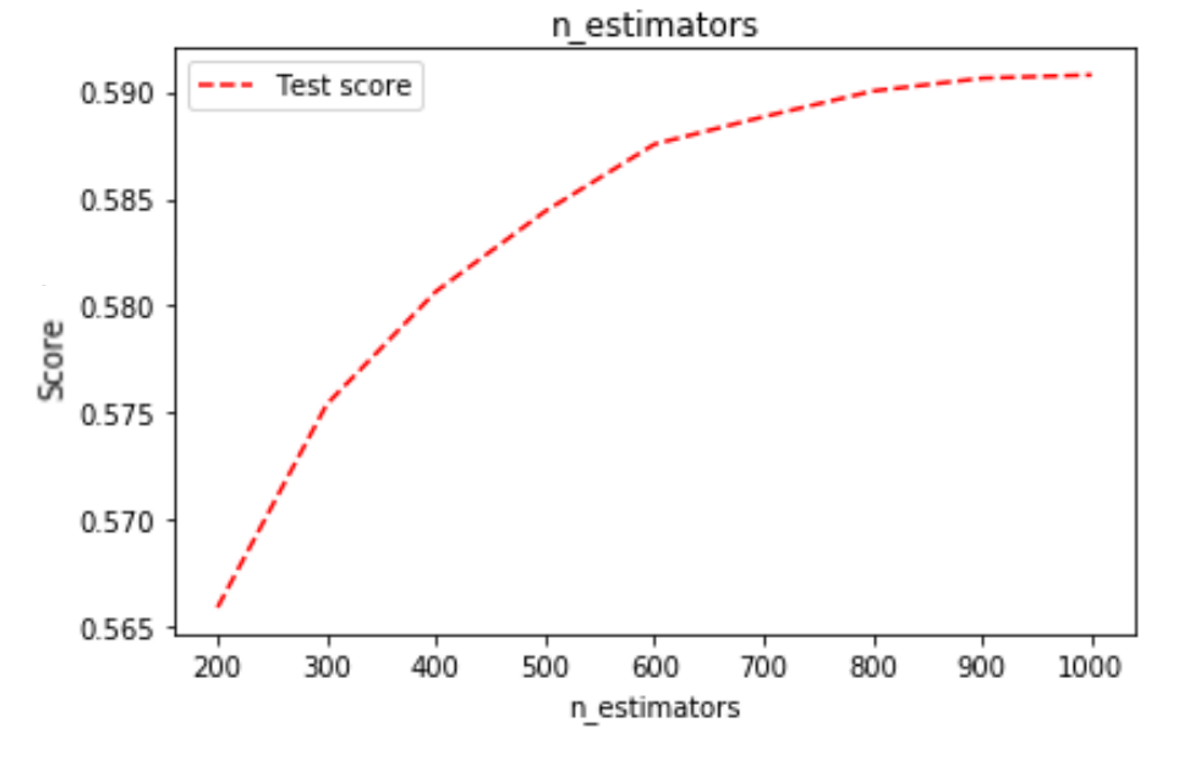
1000 estimators are barely enough for it to reach the best performance. We decided to use 600 only to reduce its time complexity while keeping a decent performance.

2. Feature Selection

Feeding too much data would also cause GBM to overfit. We can set GBM’s “max_feature” parameter to "log2" to reduce the number of features it uses to train itself.

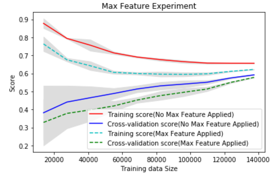
We see applying max_feature would cause GBM to perform poorly. This makes sense, as we didn’t see any overfitting issue with 600-estimator GBM.

3. Tree’s Max Depth

Decision Trees in GBM must be kept weak, thus limiting their max depth might improve the score.

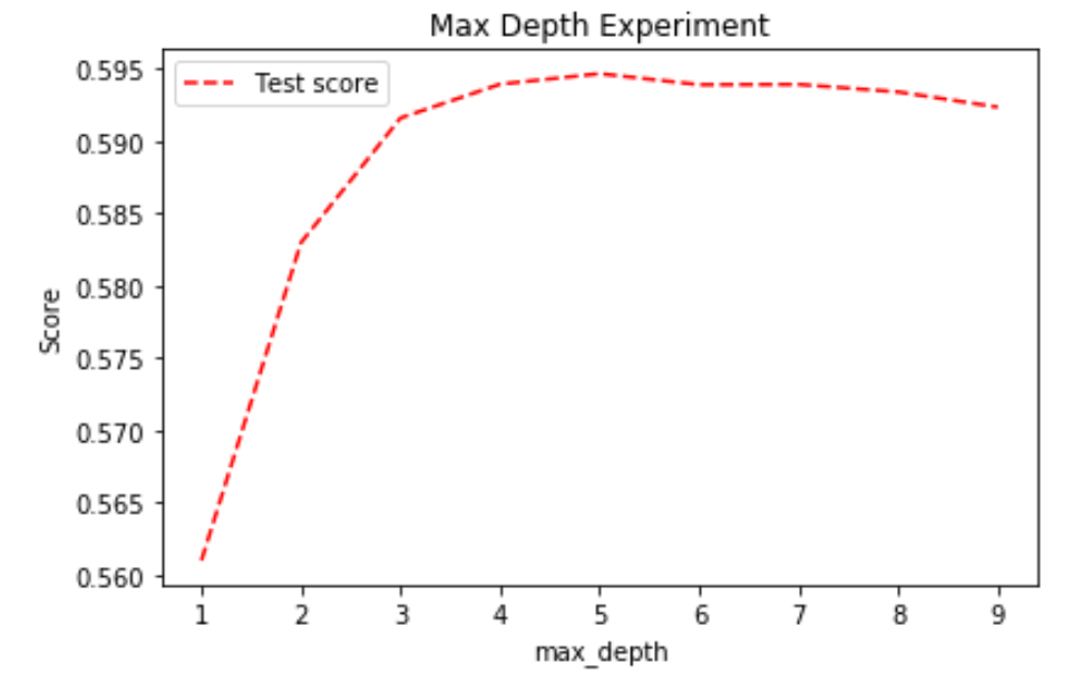
Although the Decision Trees should be very weak learners, they won't be very effective if max depth is set to too low. 5 is a good option for solving this problem.

4. Confusion Matrix

When compared to Logistic Regression and Random Forest (see star_rating.ipynb), we can see Gradient Boosting Machine is weaker in predicting 1-star and 3-star reviews. Apart from that, it has reasonable behaviour on the rest of the predictions.

5. Conclusion

The best hyperparameters for Gradient Boosting Machine are: n_estimators=600, max_depth=5

Regular NLP + Feedforward Neural Network (NN)

Due to complexity in NN, Cross-Validation is not a very popular choice and is not supported in TensorFlow Keras. Thus in experiments with NNs, we only used 100k randomly selected balanced data to train and 5k imbalanced data to validate.

1. Structure

We first researched how many hidden layers are needed.

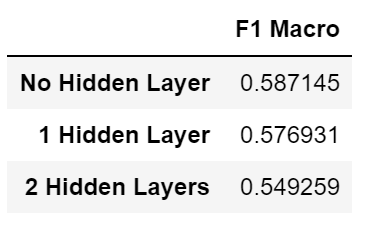
NN with no hidden layer at all achieves the best F1 Macro score. This indicates that word features and star ratings have an obvious linear relationship and NN is actually not needed to solve this problem.

However, it's too early to give up on NN yet, as we can see 1 hidden layer has a very close score of 0.577. It might be the case that, after some hyperparameter tuning NN would have a better performance.

2. Activation Functions and Optimizers

We then tried different activation functions and optimizers to compare their performance on 1 hidden layer NN

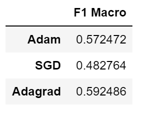
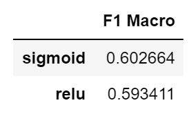
We see “Adagrad” optimizer and “sigmoid” activation function are better than the others.

We believe this is because Adagrad is a good optimizer for data with sparse gradient, which happens a lot in NLP. Adam also has a very similar performance because it's based on Adagrad.

3. Epochs

Then, we needed to find out how many epochs are needed for NN to reach its best performance.

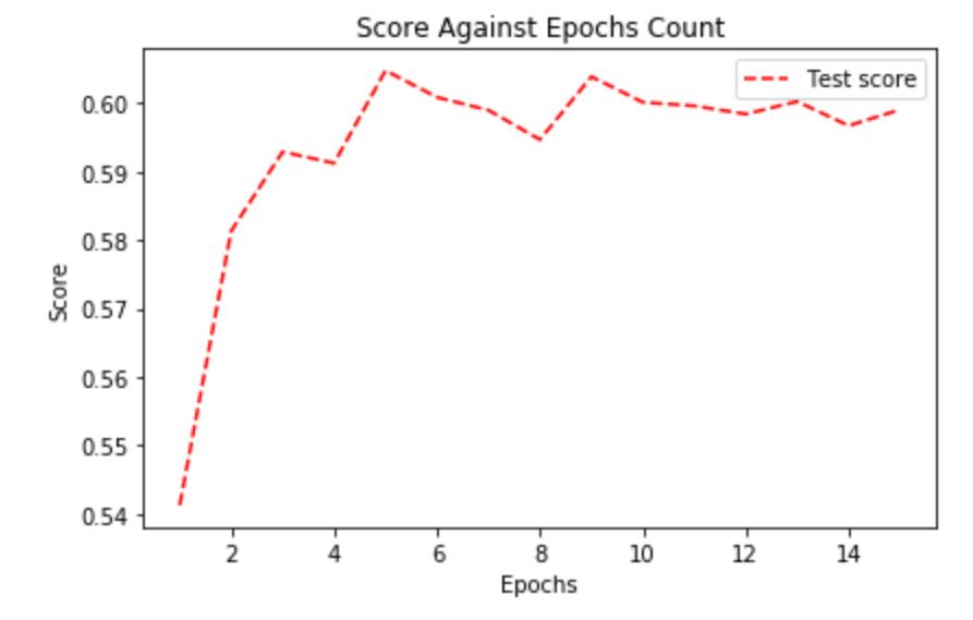
The score fluctuates a lot as we didn't use Cross-Validation here. We can see 5 epochs is optimal for our model.

4. Neurons

The number of neurons in the hidden layer is also crucial. Too few neurons would prevent NN to learn from data, whilst too many would cause it to overfit.

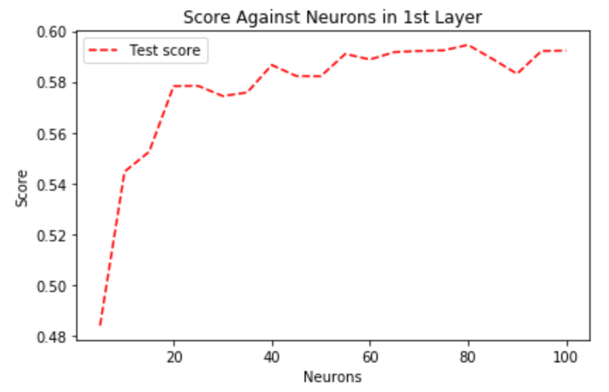
The plot shows that the best performance is reached with roughly 80 neurons.

5. Count or TF-DIF

As NN is quite different from all the models we used before, we decided to do some extra experiments with regards to NLP processors. Here we compared the effects of CountVectorizer and TF-IDFVectorizer on NN, both using uni+bigrams with vocabulary limit of 5000.

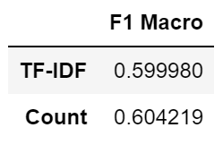
We see NN's performance is better when CountVectorizer is used. Although the difference is tiny, it would make more sense to use CountVectorizer instead.

We believe the reason for this is that, as suggested from former experiments with hidden layers, this star rating problem we're trying to solve is a very simple and straightforward problem. Thus simple techniques like CountVectorizer would not produce some complex data that can potentially confuse the NN.

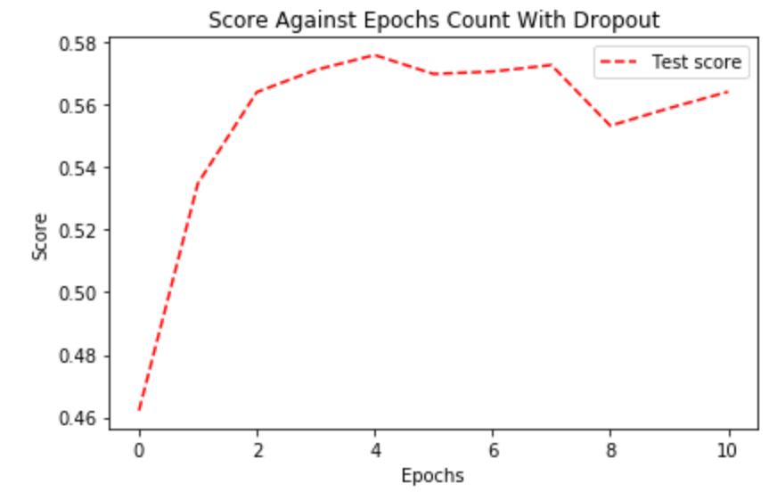
6. Dropout

Applying a Dropout layer after a hidden layer can disable some of the neurons to reduce overfitting. We experimented with it to see if it can improve our NN.

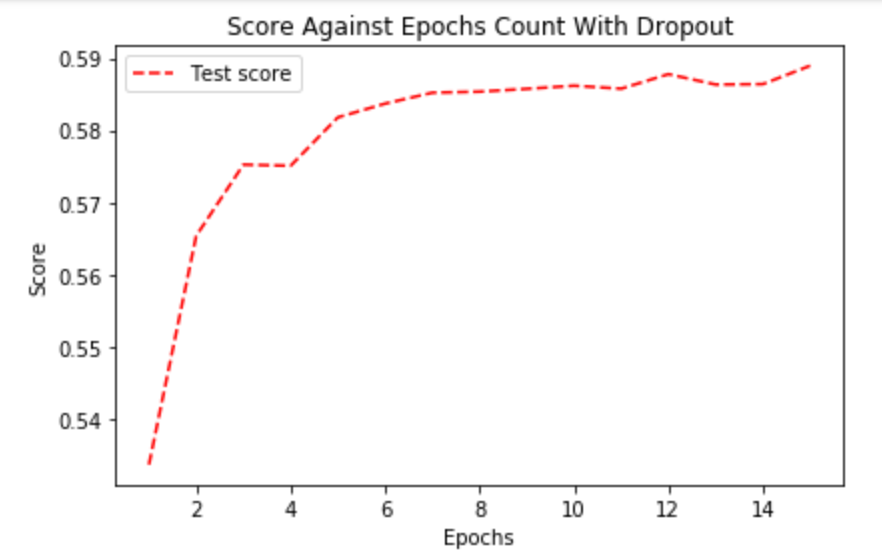
With Dropout, more epochs are needed to train NN to best performance (roughly 13). This makes sense as double the number of epochs are usually needed with Dropout. In terms of performance, it doesn't really improve the final F1 Macro score. The reason for this might be that the original NN is already very simple (as it only has 80 neurons and trained with 5 epochs) and there is nothing to regularize.

7. Confusion Matrix

Its Confusion Matrix shows the model is behaving regularly and is relatively strong. Compared to other models, we can see it's better at telling 2-star, 3-star and 4-star reviews apart.

8. Conclusion

Best settings for regular NLP Processor + Feedforward NN are: CountVectorizer (uni+bigram with 5k vocabulary limit), 1 hidden layer with 80 neurons and activatio=sigmoid, optimizer=”Adagra”, epochs=5

Word Embedding + Feedforward Neural Network

1. Vocabulary Limit

Firstly, we found out the optimized vocabulary limit for the tokenizer. Unlike regular NLP vectorizer, tokenizer doesn’t always produce arrays of the same length, thus vocab limit can be set to a larger number if needed. The experiment done here was based on the result of previous NN experiment, i.e., we used NN with 1 hidden layer which has 80 neurons.

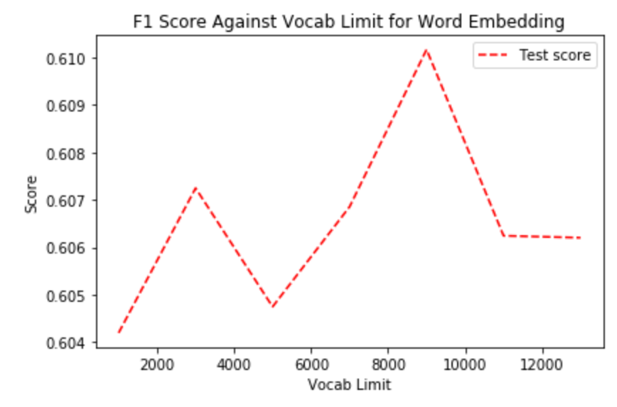
Clearly, Vocab Limit should be set to a large number for Word Embedding. 9000 would be a good number to use as it is the peak of the plot.

2. Embedding Dimension

The dimension of matrices, i.e., how long is the array that each word will be converted to, can also affect the performance significantly.

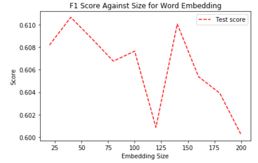
The size doesn't seem to have a huge effect on NN's performance, as the score only varies within a very small range (0.01). 50 is enough to reach the best performance.

3. Neurons

Now with Word Embedding, we have a more complex input. It's worth checking if more neurons would improve the model's performance.

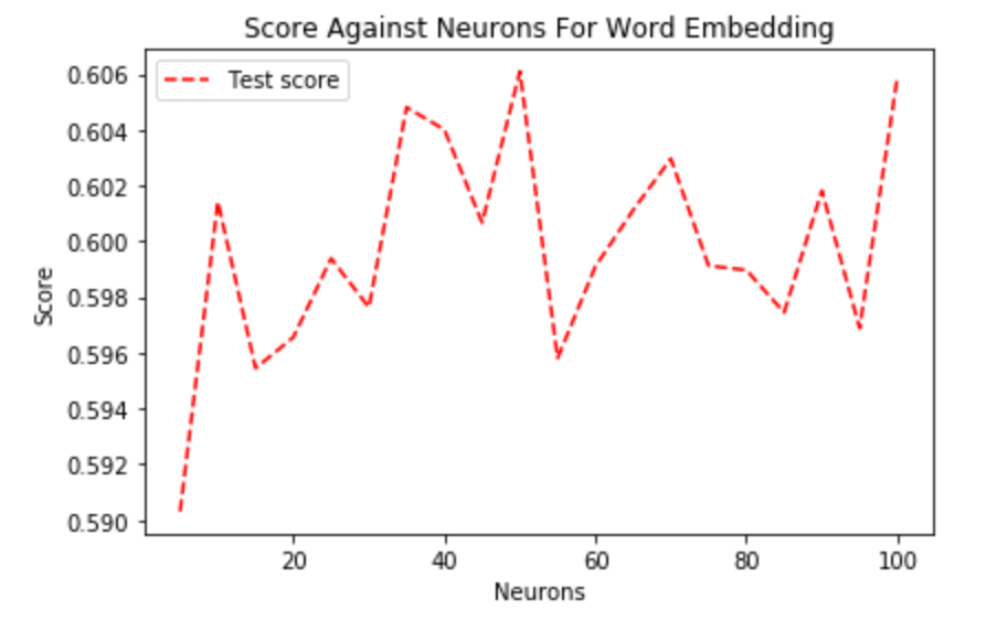
We can see even with only 5 neurons, the NN still has a fairly good performance. To reach the best score, 80 neurons is a good option and doesn't need to be changed.

4. More Hidden Layers

Just in case, we checked if Word Embedding requires more hidden layers to reach the best performance.

Clearly, it’s not the case. Sticking with 1 hidden layer only would work just fine. We believe even the form of input is different, essentially, it’s still the same problem and NNs should be identical in most aspects.

5. Dropout

Same as before, we added a Dropout layer after the hidden layer to see its effects.

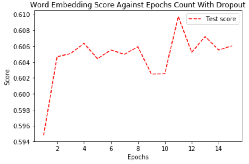
This time the result is different. The best score we reached before is roughly 0.597, whilst with Dropout, the NN is able to reach 0.606 consistently after 12 epochs. We believe it’s because the input is more complex with Word Embedding and certain regularization is needed.

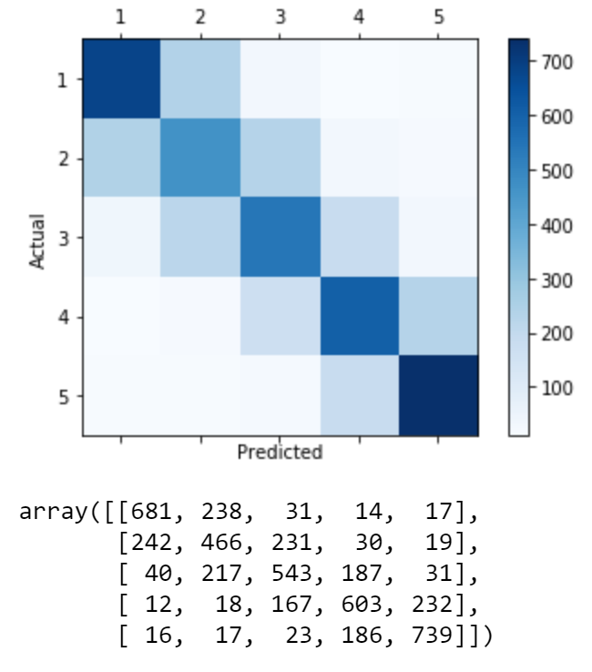
6. Confusion Matrix

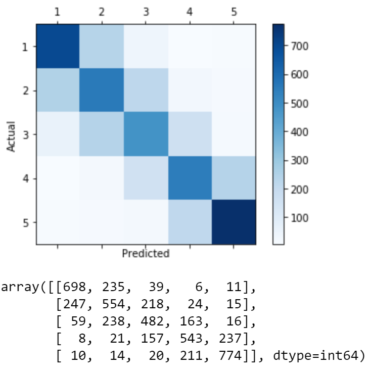
We see an extremely similar result to the one from a regular feedforward NN with CountVectorizer. In fact, they both have very similar F1 scores as well.

7. Conclusion

The best settings for Word Embedding + Feedforward Neural Network are: vocab limit=9000 for tokenizer, embedding_dim=50 for embedding layer, Dropout(0.5) after hidden layer and epochs=12. The rest is the same as CountVectorizer + Feedforward NN.

Convolutional Neural Network (CNN)

As our final experiment on star rating, we tried this extremely popular model: Word Embedding + CNN. We used the results from previous Word Embedding experiments and used vocab limit=9000 and embedding_dim=50 as optimal hyperparameters.

1. Layers

We’ve tried many recommended layouts for CNN, including Conv1D + MaxPool (0.5973), Conv1D + Conv1D + MaxPool (0.5910), Conv1D + Conv1D(more filters) + MaxPool (0.5915), Conv1D + Conv1D + MaxPool + Dense with more neurons (0.5907), Conv1D + MaxPool + Conv1D + MaxPool + Conv1D + Global MaxPool (0.5960).

Among all those layouts, the best one is Conv1D + MaxPool. However, since it’s extremely simple, we suspected that it’s just behaving similarly to Word Embedding + Feedforward NN and decided not to develop our CNN experiments on that. The second best is 3 consecutive Conv1D + MaxPool, while the last one is a Global MaxPool with a larger size. This is a very popular structure that’s found in many online tutorials and papers. Thus we decided to continue experimenting with it to see if it can give better result after tuning.

2. Dropout

The common way of using Dropout is adding it after the Dense layer (or fully connected layer). Adding it after a Conv1D layer is not recommended as Con1D layer doesn’t have many parameters and doesn’t need regularization.

However, using Dropout on the fully connected layer doesn't improve CNN at all. We believe it’s because that the CNN is already regularized by applying MaxPool and Global MaxPool.

3. Smaller Filters and Smaller MaxPool

One possible reason that restricted CNN’s performance might be the size of filters and max pools. If the size is too large, the data will be too generalized and CNN would not be able to learn any useful information. We decreased the filter and max pool size from 5 to 3 respectively to see if they contribute to the score.

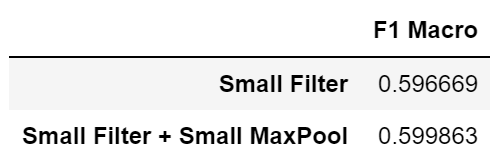
We can clearly see smaller filer and max pool size improves CNN’s performance.

4. Number of Filters

In previous experiments, we fixed the number of filters to be 128. Here we tried to test if more filters are needed.

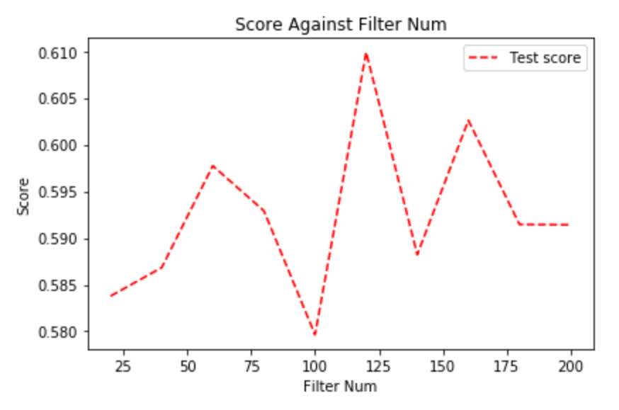
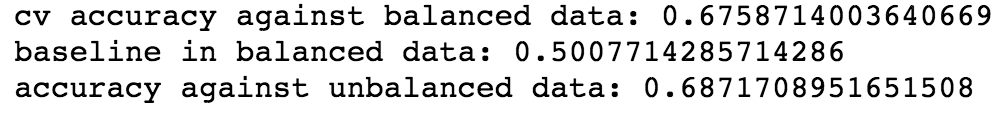
The accuracy stabilizes from 5 and more. As such we decided to use 5 and move onto finding the optimal N-estimators.

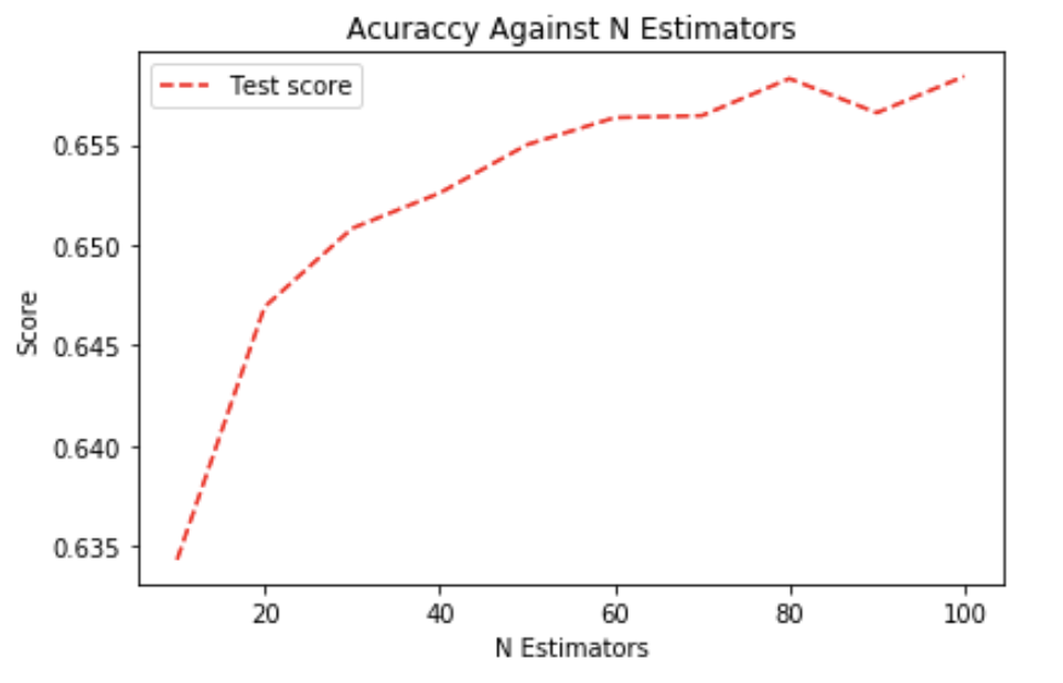
We concluded that using N estimators of 80 is appropriate because the test score becomes stable when N estimator is greater than 80 and using a bigger N estimator would only increase the processing time.

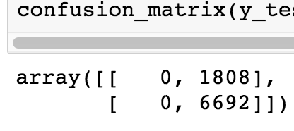
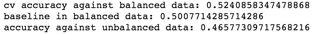
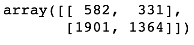
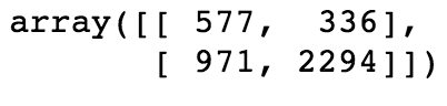
As for the model’s performance against unbalanced data:

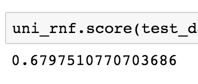
It performs similarly to logistic regression, but also similar to logistic regression it fails to beat the baseline of 0.79.

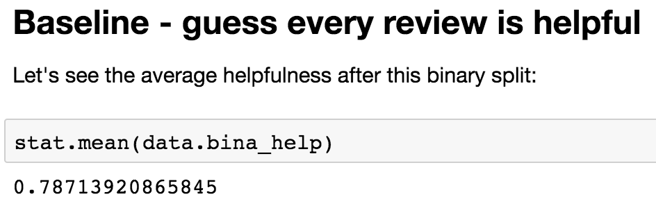
Conclusions

No model was able to beat the baseline. Ratings and bag of words were much better indicators than length however.

We concluded that such split of helpfulness data into binary classes probably ruins the remainder of the weak correlation between the features and the models- on the contrary binary rating problem had a similar baseline but had accuracies of 90%.

We talked with our client about these results, and also concluded that reviews with only 1 vote that are 100% helpful are quite unlikely to actually be that helpful, it could’ve been down to chance that one person just happened to like that review. On the other hand, if a review has many votes and a high resultant helpfulness percentage then it means that many people think this review is helpful, meaning it’s very likely to actually be helpful for all other users on the website.

Filtering out reviews with few votes causes an issue of not having enough data to train the models on the other hand. As such we decided with our client to use sample weights - when training each review’s significance on the model’s loss function will be weighted by the number of votes it has.

Regression for Helpfulness

When moving onto regression, we decided to use the things we learned when solving the binary classification problem and more or less assumed similar behaviour for bag of words and features.

As such:

• We decided to focus on Bag Of Words and ratings because length never had much impact on performance (it was negligible compared to the other 2 features).
• For bag of words we agreed to simply use 5000 words and bi+unigrams as when doing the binary problem we’ve seen that with appropriate regularization, ngram range doesn’t really matter and as long as we use more than 3000 words it should be fine so the combination we use is a jack of all trades in theory.
• We agreed to universally use vote counts as sample weights in every model for training, as we concluded that reviews with more votes should be treated with more importance.
• To measure performance we discussed with our client and decided to use mean absolute error with vote sample weights. This is because if we use weights for training in cost functions, it is irrational to judge a model by testing without the weights.

The baseline for regression:

Can be achieved by just predicting the mean helpfulness value for given rating.

Bear in mind this is mean absolute error so the lower the better.

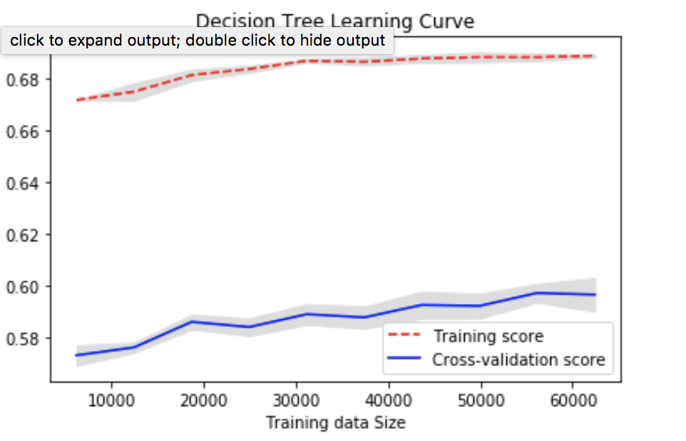
Decision Tree and Random Forest Regressors

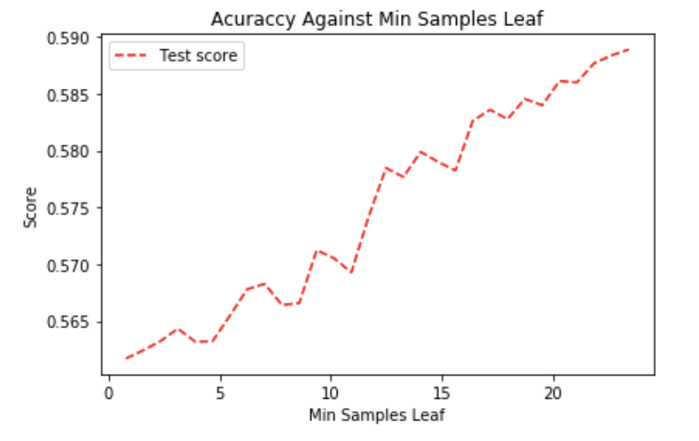
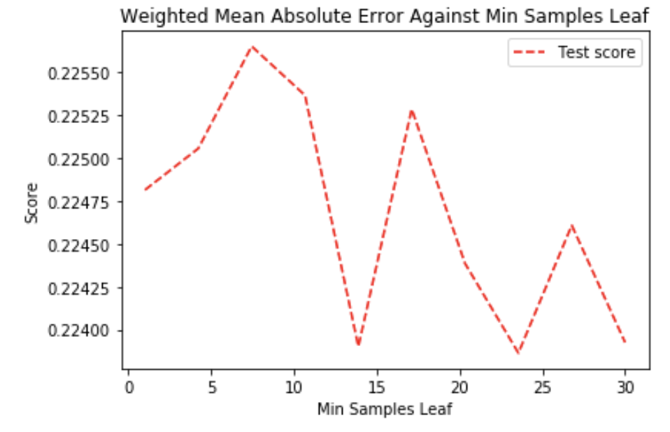
Naturally, we start with Decision Tree and look for optimal min samples leaf:

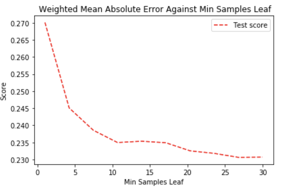
Mean absolute error decreases when min sample leaf increased. The model overfit for small value of min sample leaf, it focused too much on the noise in the data, that's why the mean absolute error is quite high. It seems that using sample leaf of 30 gives the smallest error (on graph 27 seems best but that's likely due to deviation in results).

Nevertheless, so far this is still worse than baseline.

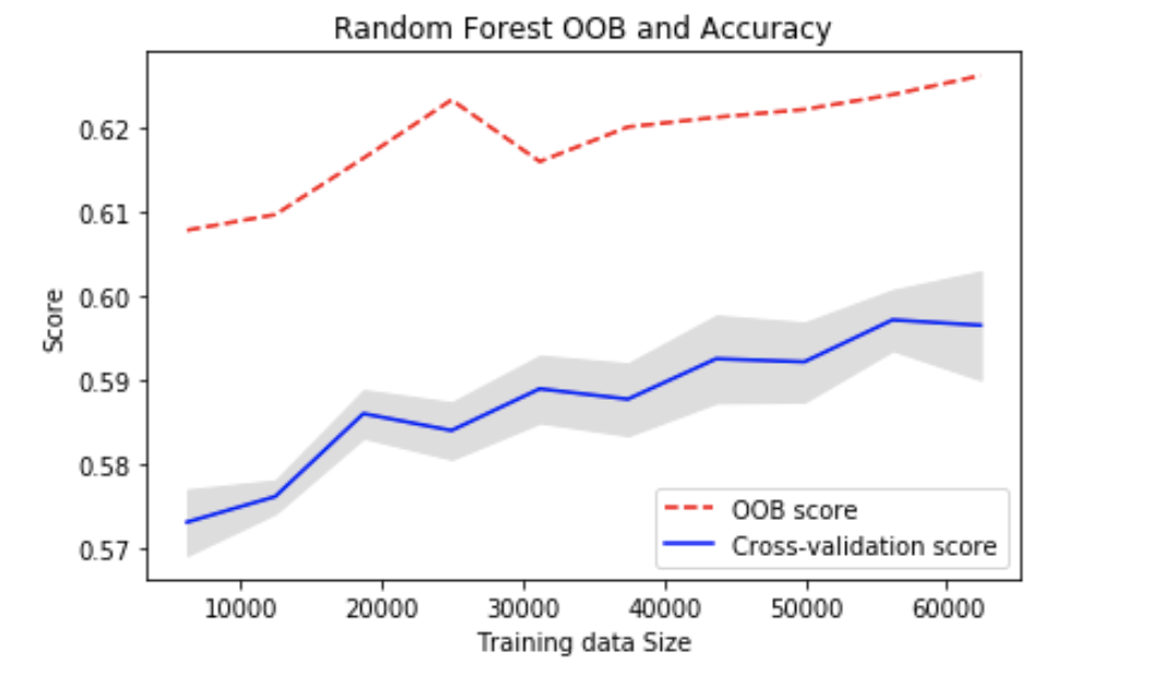
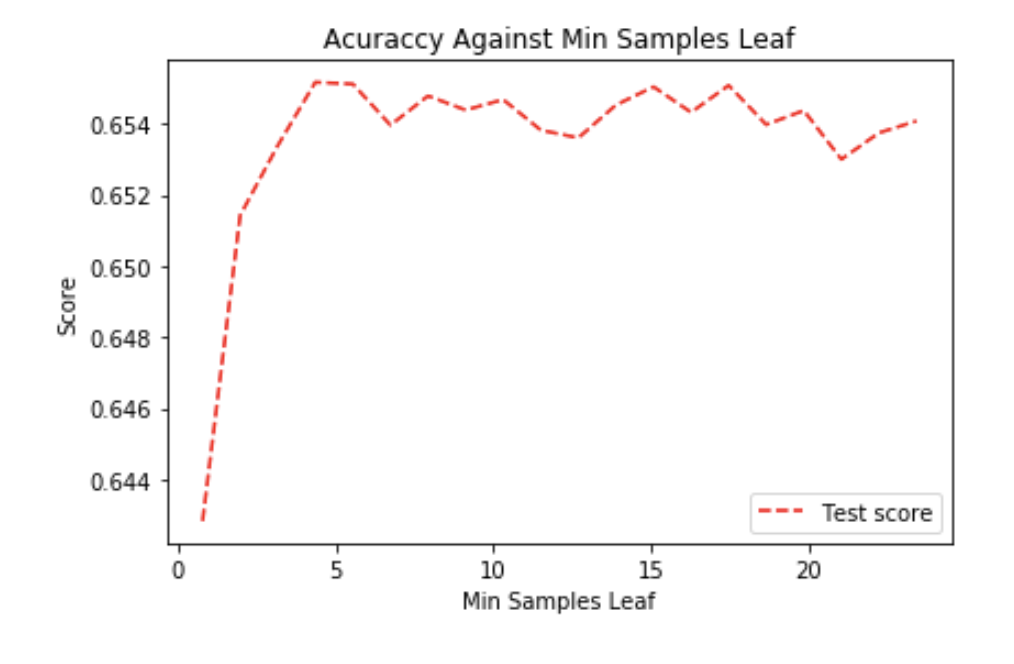
Now let’s see the random forest. We’re gonna check the min sample leaf again:

The zig-zag pattern is because of the scaling of the y-axis (range is about 0.001). A smaller leaf makes the model more prone to capturing noise in train data, it won't overfit for the random forest model because it builds multiple Decision Tree and amalgamates them together to get a more accurate and stable prediction.

It seems that there is no relationship between min samples leaf and the error so let's just leave it at the default value.

Below is the graph for N-estimators:

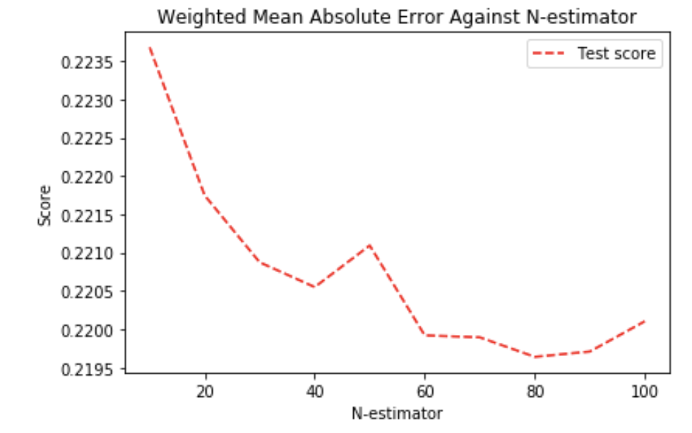
We can see the overall trend of more n-estimators being beneficial, although we can also see quite a considerate deviation on the graph.

It seems that using N-estimator of 80 is reasonable considering that using more than 80 seems to have a negligible effect compared to the error deviations.

Summary:

• Decision Tree is quite poor.
• After tuning, Random Forest beats the baseline at 80 N-estimators.

Linear Regression

The problem with linear regression was that the helpfulness problem needs values between 0 and 1 inclusive whereas the equation y = mx +c can output any real value outside of the interval [0,1]. As such we had to experiment with various functions that can be used for the mapping of y values.

1. Ratings alone - Unbounded y=mx+c model

We first decided to just try the unbounded linear regression (y = mx +c where x is rating) because despite the flaws it still can work well:

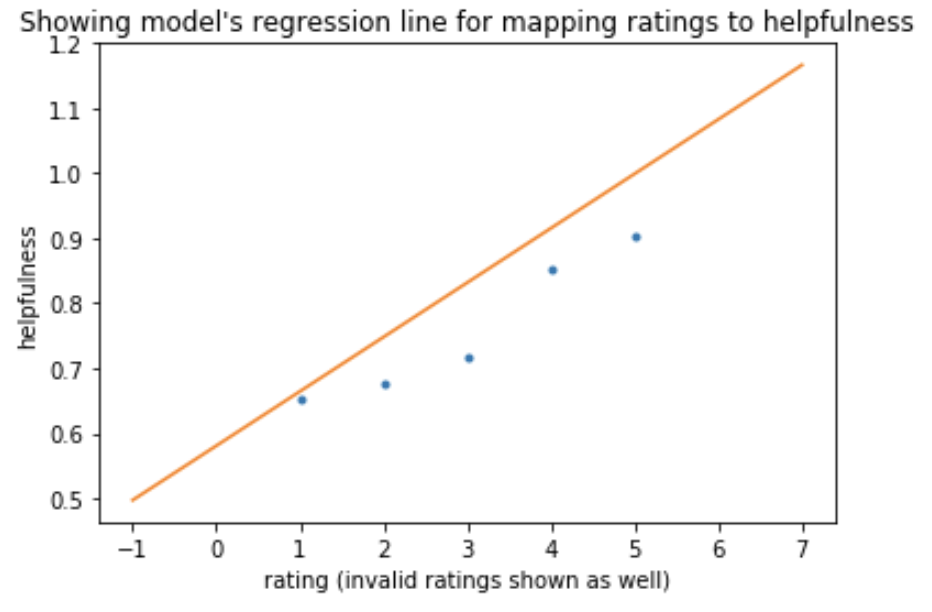
The model beats the baseline.

The graph shows that the model correctly found a positive correlation between the rating and the helpfulness. It also shows however that the model can easily yield invalid output when the rating is 6 or 7.

Of course it is impossible to have a 7-star rating, however this does show that with other models like bag of words there may be issues if the input is extreme.

2. Ratings alone - Clipping erroneous values to 1 and 0

This means that if the internal y=mx+c function outputs a value >1 it is mapped through a clipping function that will set it to 1 (and 0 for output <0).

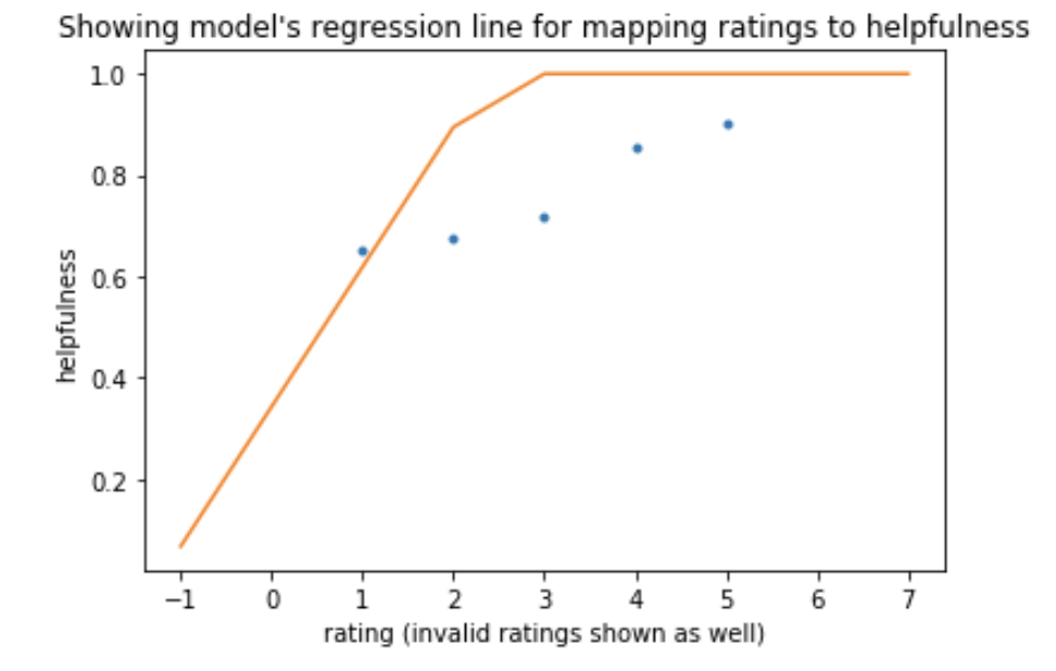
We found clipping to be slightly better than having an unrestricted linear regression.

The model has learnt to use a steeper gradient and make use of the cap for 3+ star rating.

3. Ratings alone - Sigmoid

You could argue that instead of mapping onto sigmoid we could’ve just used logistic regression from libraries, however logistic regression is for classification problems - It can output probabilities which fits our problem perfectly, but the true values of y have to be binary rather than continuous.

The sigmoid function yields roughly the same result as 'clipping', however, it is much more consistent in producing good results, unlike clipping which can get stuck if the initial weights are unlucky.

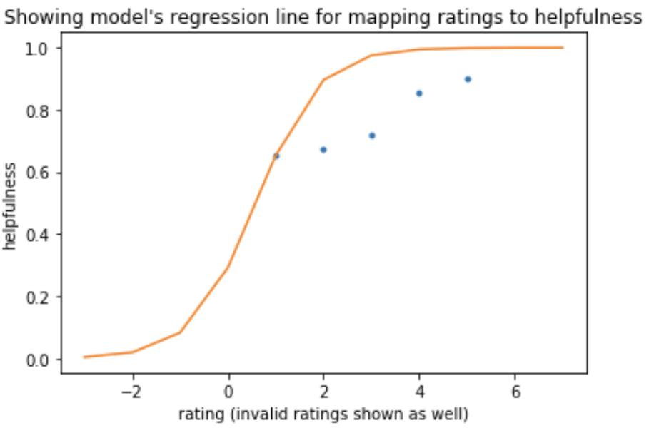
As such we decided to use sigmoid when experimenting with bag of words.

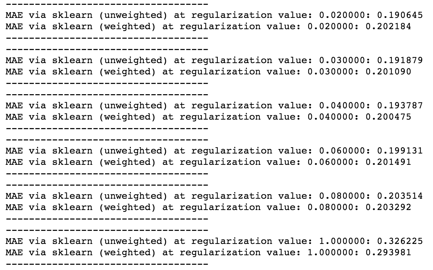
4. Bag of words + ratings

We experimented with L1 and L2 penalties. L1 yielded the best improvement over lack of regularization:

For context, these are unregularized MAE scores:

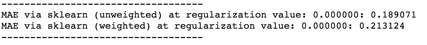
You can see an improvement of about 0.01 for best regularization value. Any bag of words combination turned out to be worse than sigmoid ratings however.

5. Conclusion:

For linear regression, it’s best to just use ratings and sigmoid function for restriction of outputs.

Feedforward Neural Network

Same as the other experiments, we randomly selected 100k reviews to train and 5k to validate. The selected reviews all have at least 1 vote. Both review text and star rating are used as features, while the vote counts are used as sample weights.

1. Hidden Layers

We tried different numbers of hidden layers to find out the optimal structure.

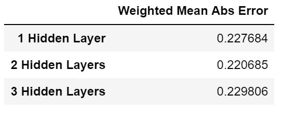
We can see that NN with 2 hidden layers has the best performance with an error of 0.221. Although the difference between each model is small, we decided to use 2 hidden layers because it seems somewhat better than the other 2.

2. Losses

We tried different loss functions.

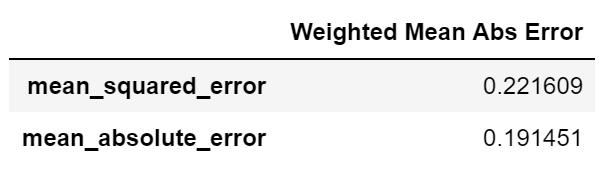
As expected, if mean abs error is used as the loss function, the mean abs error on validation dataset will also be optimal.

3. Activation Function

We then tried two popular activation functions for the hidden layer.

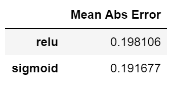
Similar to staring rating problem, sigmoid seems to be slightly better than relu.

4. Neurons and Epochs

We trained many NNs with a different number of neurons on their hidden layer and recorded their mean abs error at different epochs.

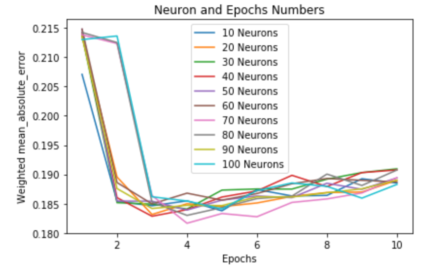
We can see that some neuron networks get stuck for 3 epochs in some local optima of 0.213. However they recover and join all other neuron counts in the top performance of around 0.185 - in fact in this graph specifically, it's 70 neurons being best and they also got stuck for 3 epochs.

We ran this graph multiple times, and we decided to use 100 neurons because it was the most stable model that always converged within 4 epochs (sometimes the models took more than 4 epochs to converge).

5. Dropout(need to be updated)

We also tried applying Dropout.

It seems that the NN got stuck in a local optimal point when using dropout. (note the small change in y-axis). As such we will not use dropout.

6. Conclusion

Best settings for Feedforward Neural Network are: 2 hidden layers with 100 neurons on each layer, activation=sigmoid, optimizer=adam, loss=mean_abs_loss, epochs=4

Conclusion

Star Rating

After finding out the optimal settings for all of our models, we put everything together using the same training and testing scheme to compare their actual performances.

In this experiment, we first randomly selected 100k data from the balanced dataset, train the models and calculated their F1 Macro scores based on 10k actual testing data (those data are reserved only for final tests and have never been used before). Then, the above process was repeated for 4 more times for every model to obtain an accurate average score as well as standard deviation. Their time used for training and testing were also recorded to represent their time complexity. (Note: since some of the models support multi-cores while some don't, the training and testing times were obtained separately through running on a single-core machine.) The final results are:

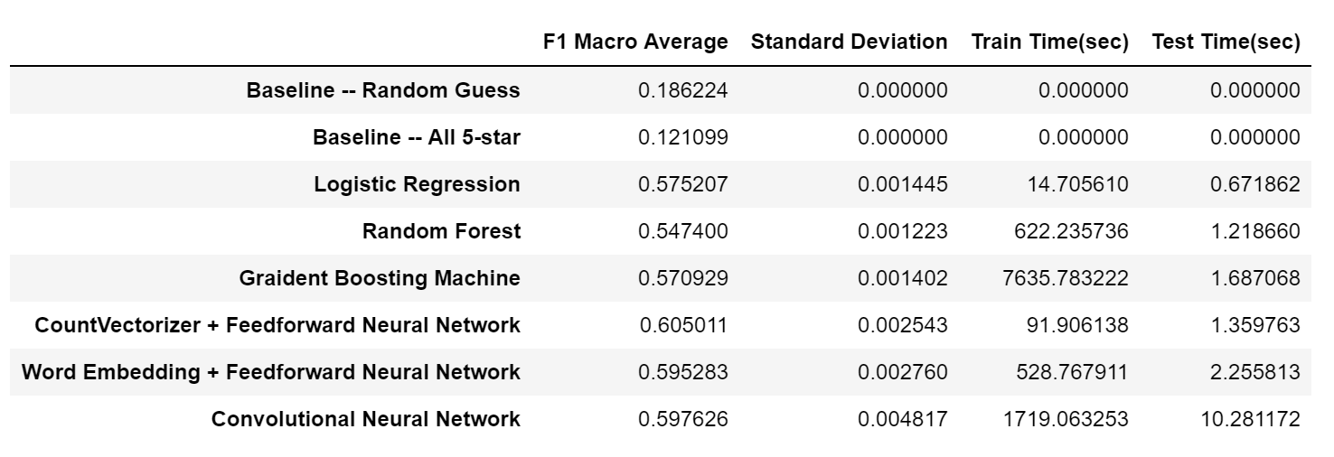
Conclusions that can be drawn from this table:

1. All of our models work properly. Compared to two baseline methods, they all show improvements of roughly 40% in F1 Macro score.
2. The worst model is Random Forest, which suggests that the star rating problem has certain linear property and non-linear models are not very good choices.
3. The most efficient model is Logistic Regression, both in terms of training and testing/actual predicting. Moreover, it has a decent score. It would be a good choice if efficiency is extremely important.
4. All Neural Network models work pretty well. Among them, the simplest Feedforward Neural Network with CountVectorizer has the best average score and least time complexity, suggesting that the nature of our problem is very straightforward and no complex techniques are required. On the other hand, although CNN's score is very close to Feedforward NN's, it has a very large standard deviation and it's very inefficient to compute.

To sum up, the star rating classification seems to be a simple linear problem. Basic "bag of words" with Feedforward Neural Network would be the best solution to solve this problem.

Helpfulness

We concluded that binary classification (at least the way we split the data) was simply a bad way to approach the problem, because the helpfulness data is likely to have simply a much poorer correlation with its features than was the case for rating prediction.

Just like with star rating, we ran each model 3 times to get an average result for each model, using 100k data for training and using the whole 10k validation dataset from our validation CSV file. We used mean absolute error weighted by vote count to measure performance.

As such, we concluded that a regression model for helpfulness values between 0 and 1 is best with mean absolute error. We tried some models for regressions, tuned the hyperparameters and put the results in one table:

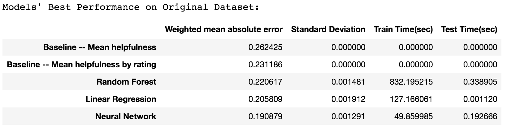
Note: Linear regression took quite long because it had a very low learning rate to ensure the best convergence. As such, it needed to train longer than necessary to get a decent result.

Conclusions that can be drawn from this table:

1. All the models listed beat the baseline.
2. Random Forest was taking quite long to compute, and yet it performed the worst out of the 3 models, which suggests that non-linear models are not very good choices for predicting helpfulness.
3. Neural Network is the best, beating linear regression which only used ratings. This means that the NN model has managed to find some useful context/correlations in the bag of words - otherwise the score would’ve been much closer to linear regression which only used ratings.

Reference

1. En.wikipedia.org. (2019). “F1 score.” [online] Available at: https://en.wikipedia.org/wiki/F1_score [Accessed 23 Mar. 2019].
2. Scikit-learn, “Linear Regression for Machine Learning,” Machine Learning Mastery, 27-Nov-2018. [Online]. Available: https://machinelearningmastery.com/linear-regression-for-machine-learning/. [Accessed: 23-Dec-2018].
3. A. Ng, “cost function,” Coursera. [Online]. Available: https://www.coursera.org/learn/machine-learning/supplement/nhzyF/cost-function. [Accessed: 24-Dec-2018].
4. A. Ng, “gradient-descent,” Coursera. [Online]. Available: https://www.coursera.org/learn/machine-learning/supplement/2GnUg/gradient-descent. [Accessed: 24-Dec-2018].
5. “Logistic regression,” Wikipedia, 09-Dec-2018. [Online]. Available: https://en.wikipedia.org/wiki/Logistic_regression#Definition_of_the_logistic_function. [Accessed: 26-Dec-2018].
6. En.wikipedia.org. (2019). “Decision tree learning.” [online] Available at: https://en.wikipedia.org/wiki/Decision_tree_learning#Gini_impurity [Accessed 13 Feb. 2019].
7. Fon.hum.uva.nl. (2019). “Feedforward neural networks 1. What is a feedforward neural network?”. [online] Available at: http://www.fon.hum.uva.nl/praat/manual/Feedforward_neural_networks_1__What_is_a_feedforward_ne.html [Accessed 26 Mar. 2019].
8. McGonagle, J. (2019). “Feedforward Neural Networks | Brilliant Math & Science Wiki.” [online] Brilliant.org. Available at: https://brilliant.org/wiki/feedforward-neural-networks/ [Accessed 26 Mar. 2019].
9. Saha, S. (2019). “A Comprehensive Guide to Convolutional Neural Networks — the ELI5 way.” [online] Towards Data Science. Available at: https://towardsdatascience.com/a-comprehensive-guide-to-convolutional-neural-networks-the-eli5-way-3bd2b1164a53 [Accessed 20 Mar. 2019].
10. Brownlee, J. (2019). “A Gentle Introduction to the Gradient Boosting Algorithm for Machine Learning.” [online] Machine Learning Mastery. Available at: https://machinelearningmastery.com/gentle-introduction-gradient-boosting-algorithm-machine-learning/ [Accessed 28 Mar. 2019].
11. Gorman, B. (2019). “A Kaggle Master Explains Gradient Boosting.” [online] No Free Hunch. Available at: http://blog.kaggle.com/2017/01/23/a-kaggle-master-explains-gradient-boosting/ [Accessed 28 Mar. 2019].