Algorithms
Description of Models
We used a selection of five machine learning regression models to experiment on and test. We decided which ones would be most useful to us for our problem of citation prediction based on the results of these experiments. This section will describe the key ideas of these models and how they work before we go on to use them in our experiments.
Linear Regression
Linear regression is one of the most basic regression models. It assumes a linear relationship between the input variables and the output variable. With a simple model only containing one input variable, this can be visualised as finding a line of best fit that goes through the middle of the data points, known as simple linear regression. This line is then used to make predictions on any other data as it maps any input to a single output. However, since we are using multiple variables for our model, we will need to use multiple linear regression instead.
Multiple linear regression uses gradient decent to find the best possible coefficients that give the “best fit”, meaning they minimise a cost function. This is an iterative process which calculates the cost function and takes a derivative to move in the direction of the minimum of this cost function. It updates the coefficients accordingly in each step to move towards this direction. A learning rate is used, this is a value that determines the size of each step. The learning rate will be decreased at each step, so the size of the steps become smaller as the solution is close. Once this minimum if found, the ideal coefficients have been found and these are used for the model. The cost function that we will be using is the residual sum of squares.
Random Forest Regressor
Random forest regression is a non-linear model that is made up of several decision trees. Decision trees are binary trees that split the data based on the features (input variables) until a “pure node”, or the desired depth, has been reached. The output can then be determined at this node.
Starting from the root, the model selects the best possible feature and feature value for the split. In the case of regression, the best possible feature and feature value will be the ones that give the highest variance reduction in the data. This can be computed as the variance in the child nodes subtracted from the variance in the parent node, where the child nodes are weighted relatively with the size of the parent node. A regression tree will be fully expanded when the desired depth has been reached, the leaf nodes can then be used to determine an output. This is done by taking an average of the data at a leaf node.
The problem with decision trees is that they can easily overfit to the training data if they are fully expanded. This means they become very good at making predictions on the training inputs but very bad at predicting data that they have not seen before. Random forest regression is used instead to solve this issue. It involves taking random sub-samples of the data set and training a several different trees with each of these sub-samples. A prediction can then be made by using all these trees to make several predictions and then taking an average of these predictions.
Extreme Gradient Boosting
The extreme gradient boosting regression model is like the random forest regressor in the way that they are both ensemble models. This model is an example of the gradient boosting model that utilises several optimisations to significantly improve performance of regular gradient boosting.
Gradient boosting works by building subsequent decision trees that improve upon each other until a cost function has been minimised. The model first starts by making initial predictions for the outputs and uses this as its starting point. The costs of these predictions are then used to build a decision tree regressor. The leaf nodes of this tree are scaled and added to the initial predictions, and the costs are calculated again to repeat the process. The factor that the leaf nodes of the trees are scaled by is known as the learning rate and it is used to prevent the model from overfitting. After all the trees have been generated, the model is complete. Predictions can then be made by combining the scaled predictions from all of the trees.
K-Nearest Neighbour Regressor
K-nearest neighbour regression is a simple regression model that uses the nearest data points to make a prediction. In the case of regression, the predicted value will be the average of the observed values of the nearest data points. The “k” refers to the number of neighbours that are considered when making the prediction.
Stochastic Gradient Descent Regressor
Stochastic gradient decent regression is like Linear regression since it is a linear model that uses gradient decent to find the best possible coefficients that minimise the cost function. The key difference is that stochastic gradient decent is used instead of regular gradient decent. The idea of stochastic gradient decent is that at each step instead of the whole dataset being used in each step of the gradient decent, a subset of points is used. This reduces the number of computations that need to be made which speeds up the gradient decent process massively.
Data
To get started with our experiments we first got a dataset sent to us by our client. This dataset was derived from the Microsoft Academic Graph which is a large knowledge graph of scholarly publications. Our dataset contains details of over 600,000 papers which we can use for our models.
We then use the title and abstract columns to convert the data into SPECTER vectors with the AllenAI public API. This uses natural language processing to convert the title and abstract of a paper into a large vector that we can use for predicting the citation count. After getting these vectors we concatenate the original dataset with them to get our dataset that we can use.
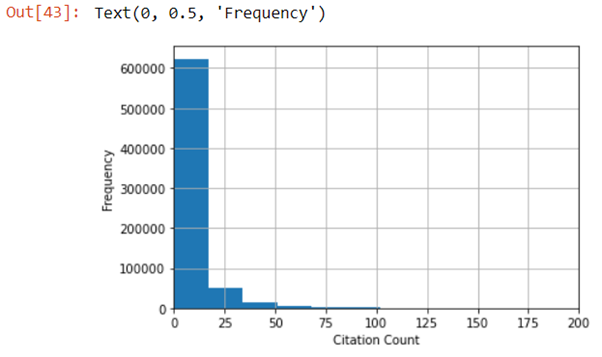
After looking at the raw dataset we found that there were some issues with it. Firstly, it is very positively skewed, because most of the papers in the dataset have a citation count of 0 which is to be expected. Also, there are some outliers with a much larger citation count than the average paper.
In order to solve these problems and make the dataset better we carried out some pre-processing steps:
- We dropped the columns in the dataset we would not be using, namely the EstimatedCitation and PaperId_x.
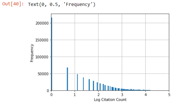
- We log transform the citation count which we will be the thing we are predicting. This will help reduce the positive skew. In particular we do log (citation count + 1) because log (0) is undefined.
- We remove the top 1% quantile of data to get rid of the outliers that have achieved an extremely high citation count.
- We remove non-English language rows since they won’t be relevant for our solution.
- We normalise the numeric columns that will be used for prediction. This helps speed up the rate at which the models train.
After the pre-processing is done the dataset is in a much more suitable state to start modelling. The data is still positively skewed but it is a lot less than before because of the log transformation. Removing the top 1% of data also helped make sure there are no more outliers.
Modelling
After processing the data to make it more suitable for modelling we made some final preparations to prepare the data for the modelling process. We first take a sample of 10,000 rows from our dataset for modelling. Using the entire dataset would be ideal since it would lead to the most well trained and accurate models however, this is not possible due to our hardware constraints as it would take too long to train the more complex models. 10,000 samples will give us a good amount of data that we can try multiple models on without taking up too much time.
We then separate the sample into our X set (the features we will be using to predict) and the y set (the value that we will be predicting). The X features consist of all the numeric features from our data set and the y set will be the log transformed value for the citation count, this is what our model will predict.
After splitting the data, the X and y arrays can now be used to train and test the models. However, in practice the test scores we will get from doing this will not be representative of the model’s true accuracy. This is because if a model overfits, it will receive a very high score since it is being tested on the training data. To avoid this, we split the sample into two further subsets, X_train and y_train to be used for training the models, and X_test and y_test to be used for testing the models. The split we decided on was 80% of the sample for training the models and 20% for testing which is a very commonly used split.
Baseline Models
Before starting to experiment with hyperparameters we decided it would be useful to establish some baselines.
We first train and test a dummy model, this is a model that just returns the mean for every prediction. This dummy model gives us a good indication for how our models should be performing, they should aim to be beating the dummy model.
We then train and test the default versions of the models to establish some baselines and compare these with the dummy model. We test the model against both the testing data and the training data to see how much each model overfits.
The metric we will be using to score our models in all of our tests is R^2 which is the coefficient of determination. At the least, our models must achieve an R^2 value of 0.3 and ideally they will be higher than this.
Dummy Model
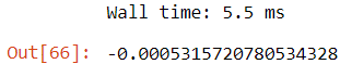
Testing the dummy model against the test data yielded a score of about -0.000532.
The score we get from this model is very poor and this is to be expected. The models that we will be using should be exceeding this score by a large amount otherwise they are clearly not suitable for the problem we are trying to solve.
Linear Regression
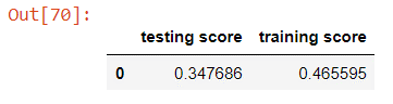
Testing the linear regression model against the test and training sets yields scores of about 0.348 and 0.466.
Linear regression performs much better than the dummy model and is very quick to train. It does very slightly overfit, since it has a higher performance when tested against the training data, however the difference is not very big and other models will most likely overfit more. Currently it meets our minimum score requirement of 0.3 but with a larger sample the score will likely increase even more.
K-Nearest Neighbour
Testing the k-nearest neighbour model against the test and the training sets yields scores of about -0.0650 and 0.330.
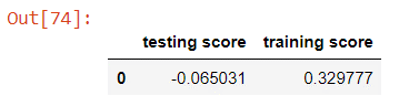
The k-nearest neighbour model performs very poorly against the test set. This is most likely because the number of neighbours that are currently being considered are too low, the default value is 5. Even so, a baseline as low as the dummy model will probably not be good enough since we will have to improve the score a huge amount just to reach our target score. This model also overfits a lot more than the linear regression model which is again because of the low number of neighbours being considered.
Stochastic Gradient Decent
Testing the stochastic gradient decent model against the test and training sets yields scores of about 0.263 and 0.364.
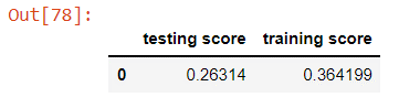
Stochastic gradient decent performs decently well and only overfits slightly. It is also quick to train like the previous models. Linear regression does have a higher baseline performance but once we begin to optimise the models stochastic gradient decent could potentially exceed the score of the linear regression model.
Random Forest
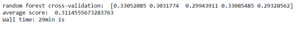
Testing the random forest model against the test and training sets yields scores of about 0.297 and 0.905.
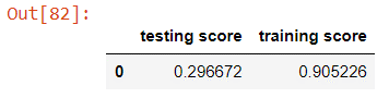
The random forest model has good performance like that of the linear regression model. Unlike the other models, it overfits a lot as shown by the training score exceeding 0.9. We will need to make sure this is fixed when optimising the model and this will most likely come down to reducing the complexity of the decision trees. It also takes a very long time to train compared to the previous model because it is a much more complex model.
XGBoost
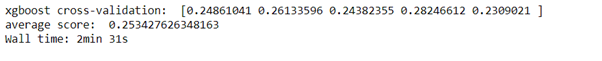
Testing the xgboost model against the test and training sets yields scores of about 0.238 and 0.951.
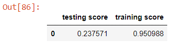
The xgboost model has similar scores to the random forest with slightly lower test performance and slightly more overfitting. This is due to similar reasons as the random forest and will need to be solved during optimisation. It takes longer to train than the simple model, but it is much quicker than the random forest.
K-Fold Cross-Validation
Our results from training and testing the default models give us a good idea of the general characteristics of the models when applied to the problems, but there are a few issues with this method. The main issue we have is that there is a trade-off with splitting the data into training and testing sets. We would like to have as many data points as possible in the training set, in order to maximise the models learning. On the other hand, we would like to have as many data points as possible in the testing set in order to get the most accurate validation when scoring the model. K-fold cross-validation is a technique we use to solve this issue without having to increase the size of the sample.
This method works by partitioning the data into k equally sized subsets and k experiments are run on these subsets. In each experiment a single subset is used to test the model and the remaining k-1 subsets are used to train the model. The cross-validation Is complete when all subsets have been used for testing (k experiments have taken place).
For our k-fold cross validation we use 5 folds to make a test-train split of 20% and 80%, the same split we used in our baseline testing stages. Using 5 folds gives us an accurate score without the time of the experiments becoming too long. The results for running cross-validation on the default models are shown below.


These scores are a more accurate representation for how are models are performing snice the entire sample is used to train and test the data over multiple iterations. We use this method in the next section for hyperparameter tuning.
Experiments (Hyperparameter Tuning)
After getting our baseline performance for all the models, we need to improve them. The performance of the models will naturally improve once we train the final versions of the models because we will be training them with a much larger sample than we are using for modelling. However, it is still necessary to improve the performance before this to get the best possible score.
The way we will do this is by hyperparameter tuning. Many of the models we are using have parameters that can be adjusted to change how the models are constructed. Changing these hyperparameters will cause the models to yield different scores which will vary from our baseline scores. Hyperparameter tuning is the process of fitting different versions of the same model with different values for the hyperparameters and testing them to find the optimal values for the hyperparameters. Finding these optimal values will make sure the models are performing the best they can.
In our experiments we are tuning the hyperparameters manually and only considering the effect of one hyperparameter at a time. Depending on the specific model and hyperparameter in each experiment, we will use a different step value and a different number of iterations. Ideally, the best way to do hyperparameter tuning would have been a grid-search which is a method that allows us to test multiple hyperparameters at a time and their affects on each other. However, this is not computationally feasible and would take extremely long for the random forest and xgboost models specifically.
Linear Regression
Since the linear regression model does not have any hyperparameters that we can tune, the baseline performance is the best performance we can get at this stage.
K-Nearest Neighbour
The only hyperparameter that will be useful to tune for the k-nearest neighbour model is the n_neighbors.
n_neighbours
The n_neighbors is the number of neighbours that are considered when a prediction is being made. In our baseline model this was set to a value of 5 which is most likely too low for our problem so increasing it should give us a better performing model.
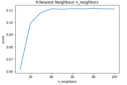
In our experiment we started with 10 n_neighbors and took steps of 10 for 10 iterations and produced the following results.
By this experiment, we can see that increasing the n_neighbors increases the score of the model until 40 n_neighbors, at which point the score levels out. The optimal value of n_neighbors is therefore 40 which gives a score of about 0.111.
Conclusion (K-Nearest Neighbour)
Since this is the only hyperparameter we will tune for the k-nearest neighbours model this will be the optimal version of our model. Even though this score is a huge improvement over the default model, this model will not be suited for our solution because the score is far too low.
Stochastic Gradient Decent
The stochastic gradient decent regressor has a few useful hyperparameters that we will be tuning, namely max_iter and learning_rate.
max_iter
The max_iter hyperparameter is the maximum number of passes that the model makes over the training data. In the default model this was set at 1000. We change this value to make sure that the model converges in the given iterations.
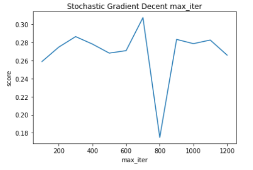
In our experiment we started with 100 max_iter and took steps of 100 for 12 iterations and produced the following results.
By this experiment, we can see that changing max_iter does not seem to affect the score since the score changes randomly. This means that the model converges before the max iterations are reached so we can keep the value of max_iter at 1000 which gives a score of about 0.272.
learning_rate
The learning_rate hyperparameter is the algorithm that is used to calculate the learning rate at each iteration of the model. The default algorithm that is used is invscaling, but we will try all the available algorithms to see which gives the best performance.
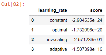
In our experiment we tested constant, optimal, invscaling and adaptive learning rates and produced the following results.
By this experiment, we can see that the invscaling learning_rate outperforms the other methods by a huge margin. We will therefore keep the learning_rate as invscaling which gives a score of about 0.257.
Conclusion (Stochastic Gradient Decent)
Since the hyperparameters that we tested for the stochastic gradient decent model were already at their optimal values, the model’s performance has unfortunately not been improved. Since the model does not meet our minimum required score, we will not be using it.
Random Forest
There are multiple hyperparameters that we will tune for the random forest regressor. These include n_estimators, max_depth, max_features and min_samples_leaf.
n_estimators
The n_estimators hyperparameter is the number of trees that are created for the random forest algorithm. The default is set at 100 which may not be enough trees for the model to make a good prediction.
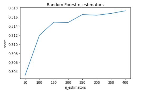
In our experiment we started with 50 n_estimators and took steps of 50 for 8 iterations and produced the following results.
By this experiment, we can see that increasing n_estimators will increase the models score. However, after about 150 n_estimators the score starts to increase at a much lower rate and fluctuate. For this reason, we will use 150 as the value of n_estimators since it is not worth increasing the value more than this since it will increase the training time a lot without increasing the score as much.
max_depth
The max_depth hyperparameter is the maximum depth that each tree is expanded. This was previously set to none, meaning the trees were fully expanded until all the nodes are pure nodes. We will most likely need to reduce this value to make the model less complex and stop it from overfitting.
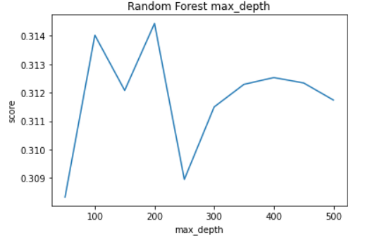
In our experiment we started with 50 max_depth and took steps of 50 for 10 iterations and produced the following results.
By this experiment, the optimal max_depth looks like 200 and a max_depth higher than that seems to consistently give worse scores, most likely because it starts to overfit. We will therefore use 200 as the value for max depth.
max_features
The max_features hyperparameter is the maximum number of features that used to split each node into the child nodes. Previously, this was set to none meaning that all the features in our input set are used by the model which is likely too many.
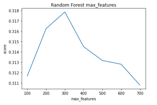
In our experiment we started with 100 max_features and took steps of 100 for 7 iterations and produced the following results.
By this experiment we can see that the score begins to increase as more features are used, until 300 features where the peak score is reached. After this increasing the amount of features yields worse performance, so we should only use a value of 300 for max_features.
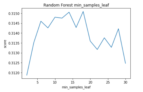
min_samples_leaf
The min_samples_leaf hyperparameter is the minimum number of data samples that each leaf is required to have on the tree. This means the model will only split a node if it leaves both child nodes with at least min_samples_leaf samples. The default value for this is 1 meaning there is effectively no minimum value enforced. Increasing this will stop the model from overfitting and potentially improve performance.
In our experiment we started with 2 min_samples_leaf and took steps of 2 for 15 iterations and produced the following results.
By this experiment we can see that the changes in score from changing min_samples_leaf are quite unstable. However, we can see that the score is the highest on average between 10 and 18 min_samples_leaf, specifically the hgihest score is reached at 18. So we will use a value of 18 min_samples_leaf.
Conclusion (Random Forest)
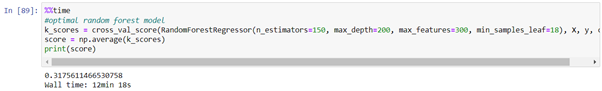
Through our experiments we found that the optimal hyperparameter values for the random forest model are 150 n_estimators, 200 max_depth, 300 max_features and 18 min_samples_leaf.
XGBoost
There are multiple hyperparameters that we will tune for the xgboost regressor. These include eta, min_child_weight and max_depth.
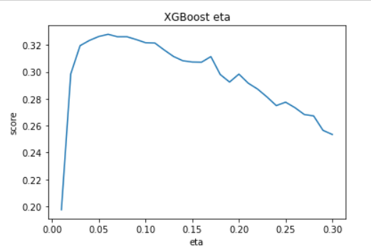
eta
The eta hyperparameter is the learning rate meaning it is the rate at which the weights shrink at each iteration of the model. The default value is 0.3 which is probably too high and may be causing some overfitting.
In our experiment we started with 0.01 eta and took steps of 0.01 for 30 iterations and produced the following results.
By this experiment we can see that the score massively increases when increasing the eta from 0.01 to 0.06, where it reaches the peak score. After this, increases in eta cause a gradual decline in score probably because the model starts to overfit. So we will use a value of 0.06 for the eta, giving a score of about 0.328.
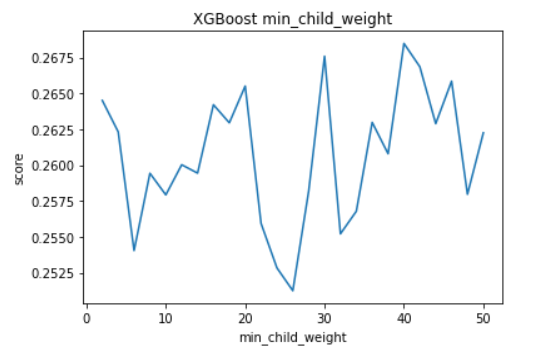
min_child_weight
The min_child_weight hyperparameter is the minimum sum of weights of all observations required in a child. This is similar to the min_samples_leaf hyperparameter for the random forest model. By default, this value is set at 1, which is probably causing most of the overfitting. We will need to increase this value to solve this and potentially improve performance.
In our experiment we started with 2 min_child_weight and took steps of 2 for 25 iterations and produced the following results.
By this experiment we can see that changing the min_child_weight shows unstable results. The fluctuations are very high on the entirety of the graph. This could be because changing the min_child_weight reduces overfitting but also reduces complexity in the decision trees causing performance to become worse. On average the higher values of min_child_weight give better scores, specifically a min_child_weight of 40 which gives a score of about 0.268, so this is the value we will use.
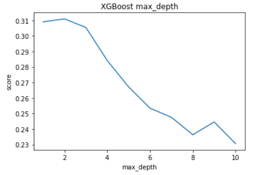
max_depth
The max_depth hyperparameter is the maximum depth that each tree is expanded, the same as the max_depth for the random forest model. The default value is set at 6 which could be too low. We will need to increase this without increasing it up to a certain amount to avoid overfitting.
In our experiment we started with max_depth 1 and took steps of 1 for 10 iterations and produced the following results.
By this experiment we can see that increasing the max_depth in fact gives worse performance. The only increase we see is increasing max_depth from 1 to 2 and from there onward any increase causes the score to steadily drop. This is most likely because we underestimated how quickly the xgboost model will overfit, so we need max_depth to be very low to reduce complexity of the trees a lot and prevent overfitting. We will use a max_depth of 2 which gives a score of about 0.311.
Conclusion (XGBoost)
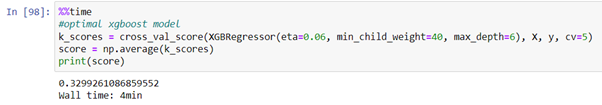
Through our experiemnts we found that the optimal hyperparameters for the xgboost model are 0.06 eta, 40 min_child_weight and 2 max_depth.
Final Conclusions
Our experiments have allowed us to decide which models are best suited for our problem and we have found the optimal values of the hyperparameters of these models.
Linear Regression
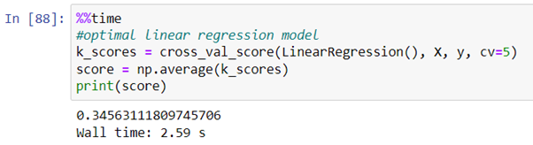
The linear regression model did not have any hyperparameters we could tune, however we will still use it in our final solution because it is our best performing model. This suggests that the data we are using to train the models has a linear trend. The optimal version of this model is therefore the default model giving a score of about 0.346.
K-Nearest Neighbour
After tuning the n_neighbors hyperparameter for the k-nearest neighbours model we found that the optimal value was 40 which gives a score of about 0.111. This score is far too low for us so the k-nearest neighbour model is clearly not suited for our problem. This is most likely because this model tends to perform worse with a large number of input varibales and we are using an array of over 700 features. So we will not be using this model in our final solution.
Stochastic Gradient Decent
When changing the hyperparameters for stochastic gradient decent we found that the baseline model already had the optimal values for the hyperparameters. The baseline model gives a score of about 0.298 which is below our minimum required score. This means we will not be using this model in our final solution.
Random Forest
Tuning the hyperparameters for the random forest model showed some noticable improvements in performance. We especially saw a good increase in performance by reducing the max_features to 300. This also made the model train much faster. Using the optimal values we can see that the random forest model achieves a score of about 0.318 which is a slight improvement on the baseline score of 0.311. So we will use this model in our final solution since it exceeds our minimum required score.
XGBoost
Experimenting with the xgboost hyperparameters showed some improvements in scores, especially tuning the eta which showed a huge increase. However, after using the optimal values we discovered that the score it gave us (about 0.305) was lower than the score we got with just using the optimal value of eta. After some further experimenting, we found that this was because the eta and max_depth parameters are affecting each other. We decided to use a max_depth of 6 (the default) along with the optimal eta and min_child_weight values. This solved the issue and gave us a score of about 0.330 which is a huge improvement on the baseline score of about 0.253. So we will use the xgboost model in our final solution since it exceeds our minimum required score.
References
1. Frost, J. (2018) "How To Interpret R-squared in Regression Analysis" [online] Available at: https://statisticsbyjim.com/regression/interpret-r-squared-regression/ [Accessed 10 December 2021].
2. Brownlee, J. (2019) "Gradient Decent For Machine Learning" [online] Available at: https://machinelearningmastery.com/gradient-descent-for-machine-learning/ [Accessed 20 December 2021]
3. Statistics Solution (2013) "What is Linear Regression" [online] Available at: https://www.statisticssolutions.com/free-resources/directory-of-statistical-analyses/what-is-linear-regression/ [Accessed 20 December 2021]
4. Scikit-learn.org (2022) "1.10. Decision Trees" [online] Available at: https://scikit-learn.org/stable/modules/tree.html#:~:text=Decision%20Trees%20(DTs)%20are%20a,as%20a%20piecewise%20constant%20approximation. [Accessed 22 December 2021]
5. Gurucharan, MK. (2020) "Machine Learning Basics: Random Forest Regression" [online] Available at: https://towardsdatascience.com/machine-learning-basics-random-forest-regression-be3e1e3bb91a [Accessed 27 December 2021]
6. Brownlee, J. (2021) "A Gentle Introduction to XGBoost for Applied Machine Learning" [online] Available at: https://machinelearningmastery.com/gentle-introduction-xgboost-applied-machine-learning/ [Accessed 28 December 2021]
7. Nvidia (2022) "XGBOOST" [online] Available at: https://www.nvidia.com/en-us/glossary/data-science/xgboost/ [Accessed 28 December 2021]
8. Stojiljković, M. (2022) "Stochastic Gradient Descent Algorithm With Python and NumPy" [online] Available at: https://realpython.com/gradient-descent-algorithm-python/ [Accessed 20 January 2022]
9. Brownlee, J. (2020) "A Gentle Introduction to k-fold Cross-Validation" [online] Available at: https://machinelearningmastery.com/k-fold-cross-validation/ [Accessed 28 January 2022]
10. En.Wikipedia.org (2022) "Hyperparameter optimization" [online] Available at: https://en.wikipedia.org/wiki/Hyperparameter_optimization [Accessed 10 February 2022]