Data Slicing Algorithms

Description

After merging data records to common categorizations, and clearing the data of obvious errors, to avoid potential reporting bias and other errors, a slicing algorithm was applied to cut out the less reliable part.

Observation

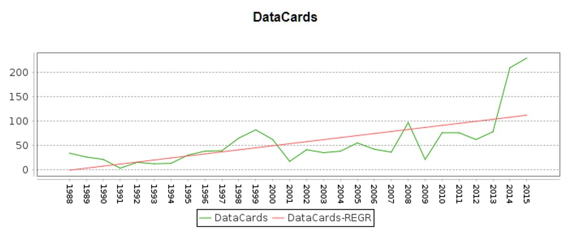
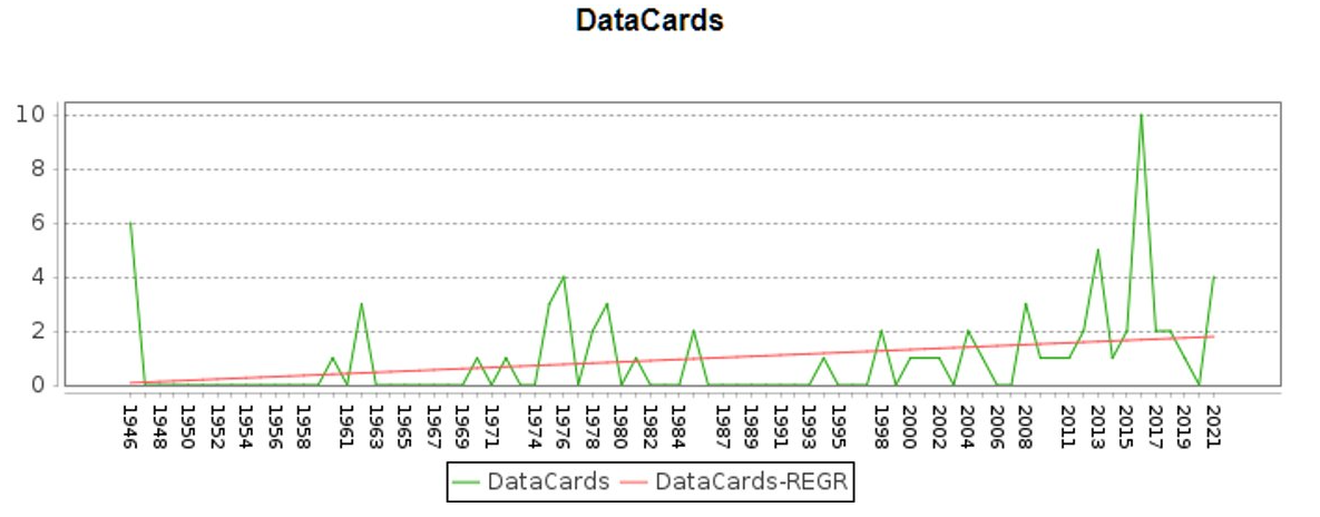
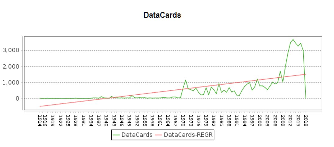
By going through the data distribution plots, we have the following observations:

  1. The number of data records varies from country to country, sometimes by orders of magnitude.
  2. The distribution of records are not even through time.​

Examples:

Assumption

The slicing algorithm is designed based on the following assumptions:

  1. The reliability and accuracy of every country increase through time.
  2. Hazards tend to be more frequently due to the global warming and climate change.

Algorithms

This algorithm monitors the gradient of the data records-time graph for every set of data, and cuts off the parts with abnormal gradients.

Evaluation

Hard to define abnormal threshold. May violate assumption one. Therefore it is not deployed.
This algorithm intends to skip suspicious parts by cutting off the first 5% records for each merged event and can be represented by the following equation:

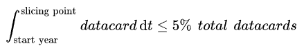
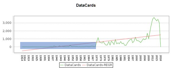
Fig.1. The first 5% records (in blue) were discarded

Evaluation

Not flexible and for data with trustful shape may reduce sample size. Ignore the content of the record, for countries including Saint Vincent and the Grenadines, the record of fatalities and affected people remains to be zero for all 10 records. This leads us to the third algorithm.
This algorithm is the extension of algorithm integration and intends to only keep the last 15 years’ record after the 21st century.

Evaluation

By combining these two slicing rules and applying one or both of them to different datasets based on their size and content, we can ensure that the data used in subsequent analyses is relatively more reliable.

Return Period Algorithms

Description

As mentioned in client requirements, the final task of this project is to generate the impact return period curves for 91 countries. The characteristic associated with the return period and normally calculated firstly is the exceedance frequency. According to Oosterbaan(1994, p.11) and Aznar-Siguan(2019, p.5), they are defined to be reciprocal to each other:

  •   (1.1)
  •   (1.2)

Where in (1.1) Tr is the associated return period of the frequency of exceedance of the impact x exceed a reference threshold Xr. Similarly, in (1.2) v(x) is the exceedance frequency of impact x, T(x) is the equivalent return period.

To calculate the frequency of exceedance, Oosterbaan(1994, p.10) introduces the ranking algorithm, in descending order for instance:

1. Rank the total number of data (n) in descending order according to their value (x), the highest value first and the lowest value last;
2. Assign a serial number (r) to each value x (x, r = 1,2,3,...,n), the highest value being X1 and the lowest being Xn;
3. Divide the rank (r) by the total number of observations plus 1 to obtain the frequency of exceedance;

Evaluation

As Oosterbaan(1994, pp.10-11) mentions, (1.3) is not an unbiased estimator and it is listed because for x close to the average, it makes little difference and the bias would be less significant and other estimators found in literature have the same issue.
 (1.3)
The reason this algorithm is biassed can be seen when dealing with events with the same impact. While ranking events by their impact, especially considering impact such as fatalities, it is not rare to have events have identical impact and by applying this algorithm they would have incremental rank, therefore they would have biassed frequency of exceedance.

Moreover, in our case, for events with different return periods, the impact varies sometimes even exponentially and x will infrequently approach to average. This makes improvement necessary.
This algorithm is an improvement of the ranking method and builds on an assumption that for years lack of record events with an impact of 0 occurred.

After ranking in ascending order, instead of assigning a rank to each event, count the frequency of events that exceed the threshold of interest by dividing the total number of events that exceed the threshold by the total number of observations. For example, if there have been 10 floods with affected people exceeding 100 in the past 20 years, the frequency of exceedance would be 10/20 = 0.5.

Once we have the frequency of exceedance, we can calculate the return period as the reciprocal of the frequency of exceedance, as shown in (1.1). For example, if the frequency of exceedance is 0.1, the return period would be 1/0.1 = 10 years.

Evaluation

In the implementation, this algorithm ensures that events with the same level of impact will be plotted at the same position, and the repeated drawing of the same point may involve unnecessary computation consumption. However, given the computational power required for additional de-duplication of the results and the fact that the largest dataset, for example, Mexico, has only 831 records, the impact of such loss on the overall time of calculation and the efficiency of the plot is imperceptible and therefore acceptable.

Conclusion

This project involves two main algorithms, a slicing algorithm for cleaning the data, and a cumulative sum algorithm for calculating the return period.

They both exclude as much erroneous data as possible and enhance the reliability of the results in the absence of further validation conditions, such as the introduction of a new database for comparison.

However they failed to address the following issues:

  1. For the overall lack of data, especially where the combined records were still less than 30, further interceptions of them produced return period graphs that were either very limited in period, sometimes with maximum return periods even less than the 10 years we were concerned with.

  2. For unrecorded years, it is assumed that there were no hazards or that the impact of the hazards that occurred was zero, when in fact it may be because the impact was minor and not recorded or was missing for other reasons. Given that the project is primarily concerned with these minor but frequent hazards, this assumption leads to a relatively large bias.

  3. The algorithm for calculating the return period is particularly sensitive to errors in dates, for example, the flood records for The Gambia contain 15 events with unknown years but labelled as having occurred in 1900. These records significantly pull up its maximum return period.

References

  1. Oosterbaan, R.J., Nijland, H.J. and Ritzema, H.P., 1994. Drainage principles and applications. International Institute for Land Reclamation and Improvement (ILRI).
  2. Aznar-Siguan, G. and Bresch, D. N., 2019: CLIMADA v1: a global weather and climate risk assessment platform, Geosci. Model Dev., 12, 3085–3097, https://doi.org/10.5194/gmd-12-3085-2019