Data Downloading

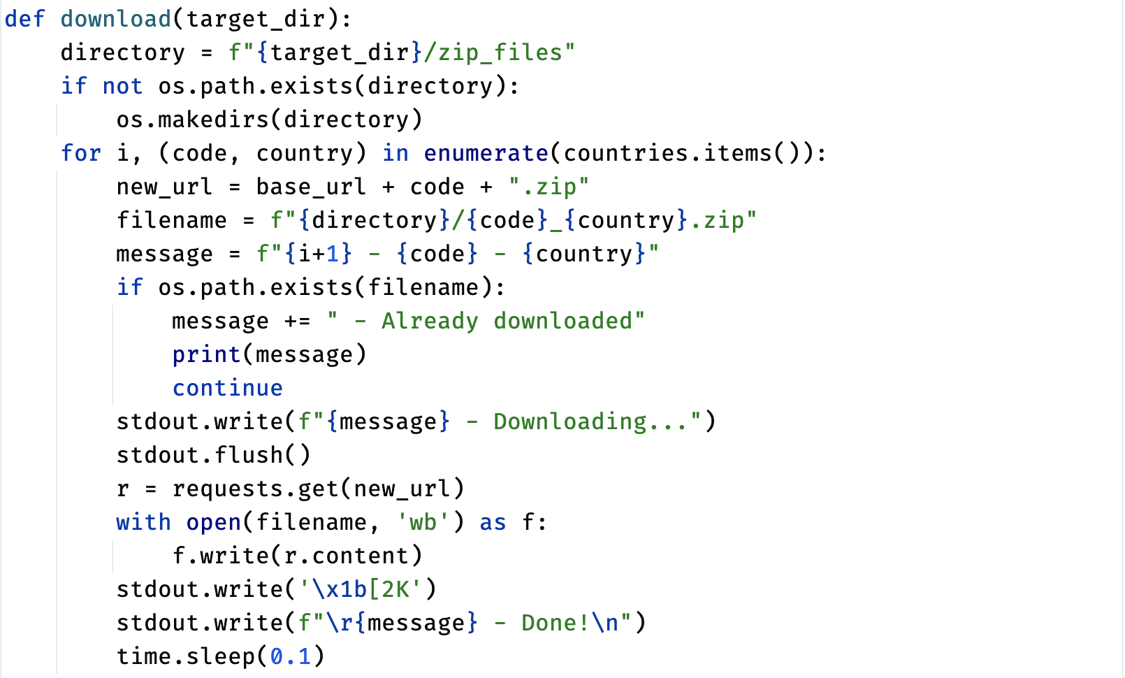
The DesInventar Dataset contains a vast amount of data related to natural disasters, across various countries and regions. Downloading this data one at a time would be a time-consuming process. To streamline this task, we used the BeautifulSoup and requests library to web-scrape the DesInventar website. As such, we were able to extract XML Files for each country and region, with the events that occurred within them.

Once we had collected this information, we were able to use DesInventar's public API to download all the files. This approach saved us a significant amount of time, not having to manually download the data for each country. Furthermore, it ensures the model can automatically update with the presence of new data.

Data Parsing

The downloaded files were in XML, as such, we had to parse them to CSV, to remove unnecessary information. This process was quite memory-intensive, particularly when dealing with larger XML files. In particular, the XML file for Sri Lanka was large and required approximately 60GB of RAM at its peak.


The heavy memory usage prevented us from parsing on our personal computers. Machines available at the university labs provided 128 GB of RAM which we utilised. But, we were not always on campus so that was restricting. In the future, We will optimise the conversion process. Utilising chunking - which parses XML line by line to reduce memory usage. As a result, we would be able to parse much larger files without memory restrictions.

Data Categorisation

During data exploration, we saw disaster categories that were irrelevant to our research. These categories included non-natural hazards such as accidents, chemical leaks, etc.

To do this, we first identified the categories that we wanted to keep and those that we wanted to remove. Then, we wrote a script to remove the unwanted from the CSV files.


We saw that some disasters had different translations and spellings, which needed merging. For instance, we noticed events such as "Light Flooding" and "Falsh Floods" in the dataset. We identified those referring to the same disaster and merged them into one category e.g. Floods. Subcategories were also labelled in French or Spanish instead of English. To ensure consistency across our dataset, we translated these into English.

This step was time-consuming having to use manual filtering to categorise events. But, this step allowed us to maintain consistency across the dataset, so was crucial.

Data Slicing


When first analysing our dataset, we noticed many inconsistencies and inaccuracies. Most significant problems include missing values and random entries. Having, known inaccuracies would diminish the result of our analysis and visualisation

To address this issue, we decided to remove the values that were very inaccurate from our dataset. We had justified assumptions about the data, so we could remove inaccurate values. The most important assumption we made was that the data quality improves with time. This assumption is valid because technology has improved - resulting in better data collection.

We implemented the 5% slicing rule, due to reasons that can be found in our Algorithms section. Essentially, this allowed us to exclude the highly anomalous results which included random inaccurate years in the data.

We gave users the choice of only including data from the last 15 years. This rule was implemented to focus our analysis on more recent events that were likely to be more reflective of current conditions. Furthermore, we wanted to ensure the reliability of our data. To implement this rule, we added a parameter to our data processing script that allowed users to specify a time frame for the data. Users could choose to include data from the entire dataset or only data from the last 15 years.

The rules we set for slicing are highly modifiable to ensure extendability and it allows for changes to be made based on different data sets.

Data Aggregation

During our data exploration process, we identified that some events in our dataset were closely related in terms of location or cause and effect. These events were separate entries in our dataset which could affect our analysis if treated as independent events. To address this issue, we implemented a data aggregation technique where we combined events that were within the same region and consequences of one another. These events had separate data cards, but they should have been a single event that caused other events.


By combining these related events into a single entry, we were able to more accurately reflect the true impact of the event on the affected region. If we had treated these events as separate, it would have inflated the number of events in our dataset, resulting in a higher frequency of events but with lower impacts. Combining these related events, we reduced the frequency and increased the overall impact of the event in our analysis. Combining those events reflects the cause and effect of the event more accurately.

Data Analysis

For the implementation of the analysis, we followed a paper from CLIMADA, which we used to do the empirical analysis using the method specified in the Algorithms section. This subsection calculates the return period and gets an impact based on rankings.

Data Visualisation


Our final task with the analysis performed was the ability to visualise the data. One of the key features we included in our plots was the ability to highlight specific return periods (1, 3, 5, and 10) that our client requested. Return periods estimate the likelihood of an extreme event occurring in a given time frame. For example, a return period of 10 years means that there is a 1 in 10 chance of the event occurring in any given year.


To generate plots for specific return periods, we used a Python plotting library called Matplotlib.Pyplot. We created a function that took the results from our analysis as input and generated a plot with the specified return periods highlighted. By including these specific return periods in our plots, we were able to help our clients better understand the frequency and magnitude of extreme events in their region of interest.

Overall, generating graphs allowed them to visualise the likelihood of extreme events occurring in a region and take appropriate actions to mitigate the risks associated with these events, as compared to tables in which you can not see the trends.