Typical use cases include:
- Determining quality of food stuff
- Monitoring air quality
- Breath analysis for medical conditions
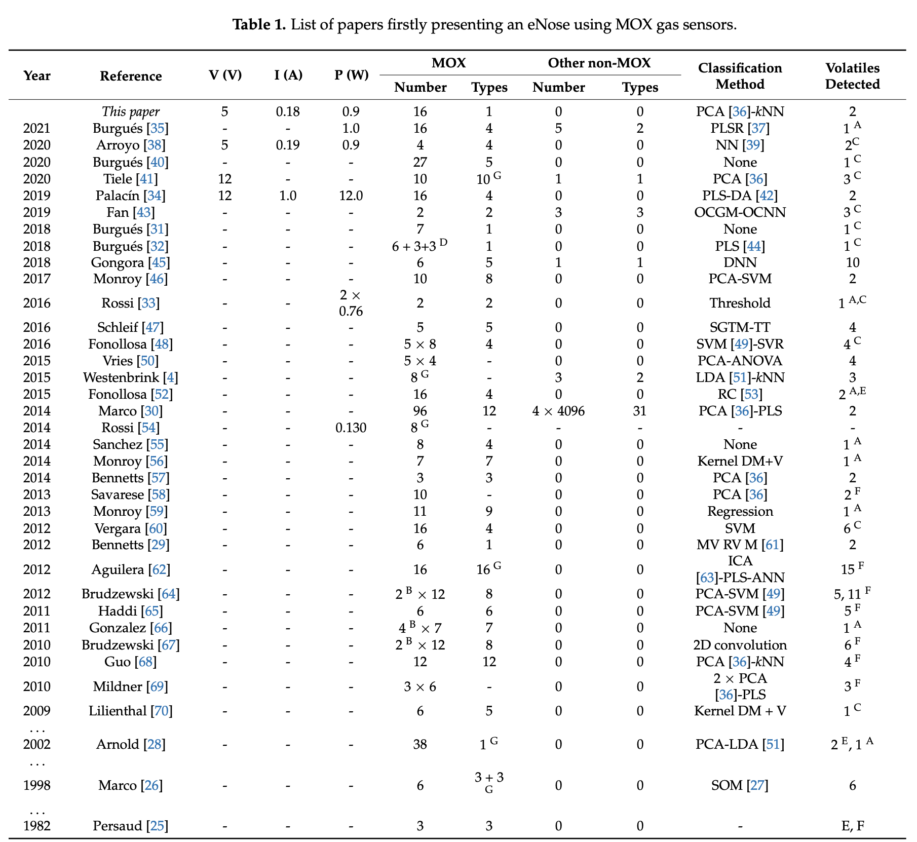
Figure 1: Previous research on MOX sensors used as "eNoses"
MOX sensors are highly sensitive but have poor selectivity. As a result, discriminating among several chemicals, or between targets and backgrounds, becomes difficult. [1]
Instability, Drift, and Variability between Sensors
Typically, using a single sensor for detection is generally avoided, as they have the tendency to drift over time, leading to inaccurate readings and need for frequent recalibration. Our observations confirms this, as in the same setup and experiment configuration and lead to wildly different results on different days. Most setups involve an array of sensors [2]. As a result, classification tasks are typically only limited to binary or few classes.
Burnouts
The sensor can also be prone to burnouts when too high of a temperature is sustained for extended periods of time, or when there is insufficient cooldown time between measurement cycles. For our preliminary experiments, 3 sensors were burn out even when operating between the recommended temperatures of the manufacturer, likely due to long experiment runs with minimal cooldown in between, yielding abnormally high levels of resistance in stale air. However, as the sensor requires a stabilisation period, cooling down for too long will also lead to inaccurate readings. One of our major challenges is to find through trial and error a suitable measurement frequency which yields sufficient cooldown time to protect the sensor without sacrificing the temporal resolution necessary for classification tasks.
Hotplate Temperature
Classification performance are also known to be effected by the configuration of heater temperature and frequency, modulated by a balance of gas adsorption and reaction on the surface of the hotplate. If the frequency of the heater voltage is too high, the surface temperature of the sensor could not keep up with the variation of the heater voltage. However, if the frequency is too low, the sensor changes slowly and tends to reach its equilibrium response, similar to a constant temperature mode. In this case, the nonlinear features of sensors could not be extracted and the feature dimension extracted at this constant temperature mode is unstable [3].
- Resistance readings are low when the sensor is inactive for more than an hour, hence requires some stabilisation time before every use to reach the reliably readings. The sensor can even miss a few readings when the hotplate fails to reach to desired temperature within the given duration during measurement cycles.
- The sensor can begin to drift up in resistance readings if it has undergone extensive periods of measurement at high temperatures without cooldown. This burnout is irreversible, where the sensor will continue to have unreliable readings even weeks after and become insensitive to gas exposure.
-
The setup required balancing the initial stabilisation time necessary to get accurate readings and the cooldown period, necessary to prevent sensor burn out through continuous data collection.
- We observed that after hours of sensor inactivity, 30 minutes of stabilisation is required, with 100 seconds of stabilisation before every measurement cycle and 10 seconds cooldown between measurements.
- 100 seconds stabilisation time is the shortest optimal time that allows us to have enough accurate readings before the scent emission to establish the baseline for correction later.
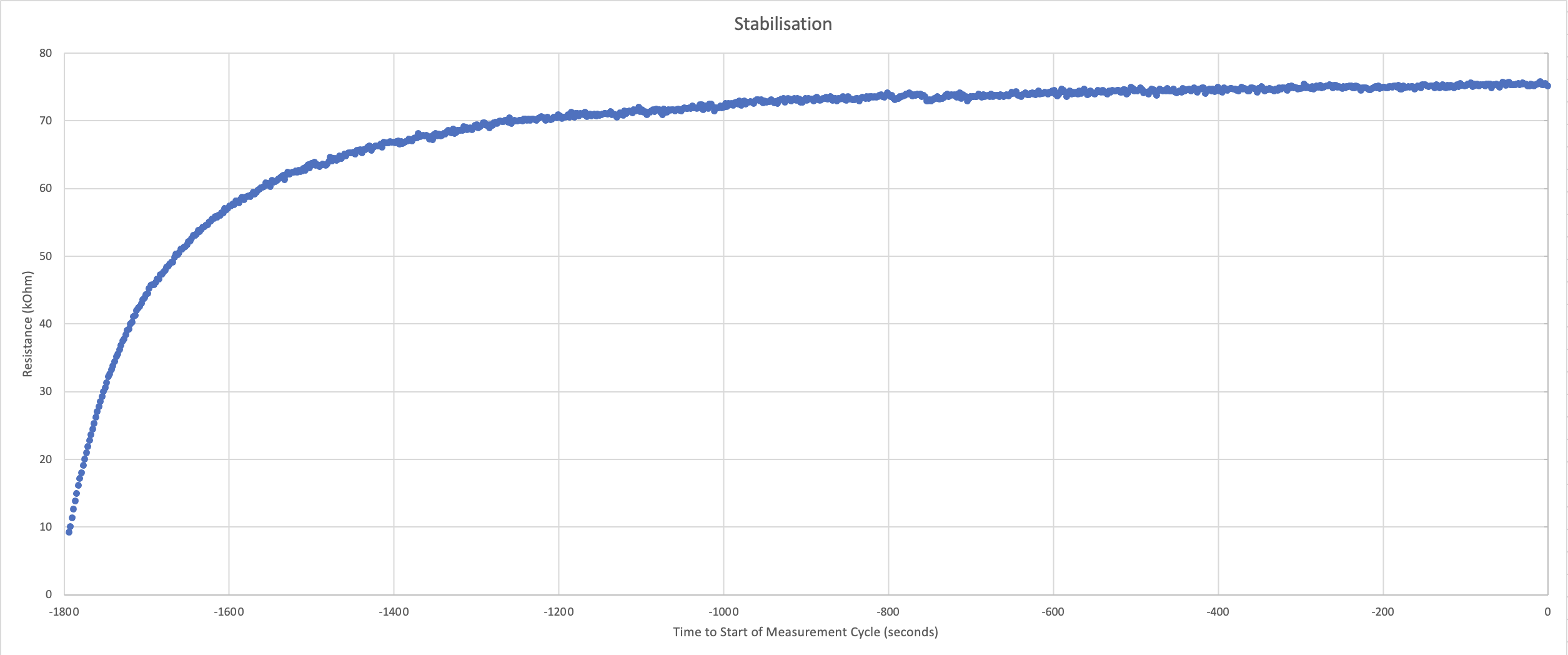
Figure 2: 30 minute stabilisation for hours of inactivity
- Using a linear increase in temperature for heater profile (220-400 with 20C steps) and a constant heater duration, we observe the magnitude (percentage decrease) from baseline resistance when the sensor is exposed to the gas, and the reaction (time at lowest resistance) differs from scent to scent.
- It showed that while the sensor had fairly reproducible responses to some scents, it was less so for the others, The swiftness and magnitude of the reaction to the scents varied greatly from session to session, as shown by left image below. This is a fairly well established problem with single sensors, hence most existing setups for classifying gasses utilize an array of 3 - 24 sensors.
- It is known that longer heater durations for each temperature is beneficial for scent discrimination. However, we observed the opposite, with the KNN performance decreasing as the heater duration increases. We also lose temporal resolution when using longer heater durations. Image below shows classification reports for 40ms (top middle) and 320ms (top right)
- The reaction to scent 2 (bottom leftmost) was reproducible across sessions with consistent magnitude and swiftness in response. This is less true for scent 1 (bottom, center left), which has great variability across sessions. It can also be seen that the two attributes (bottom, center right) do not separate the scents very well, with the exception of scent 2 and 3. Running a KNN, it achieves 73% accuracy across sessions but with increased confusion around scent 1.
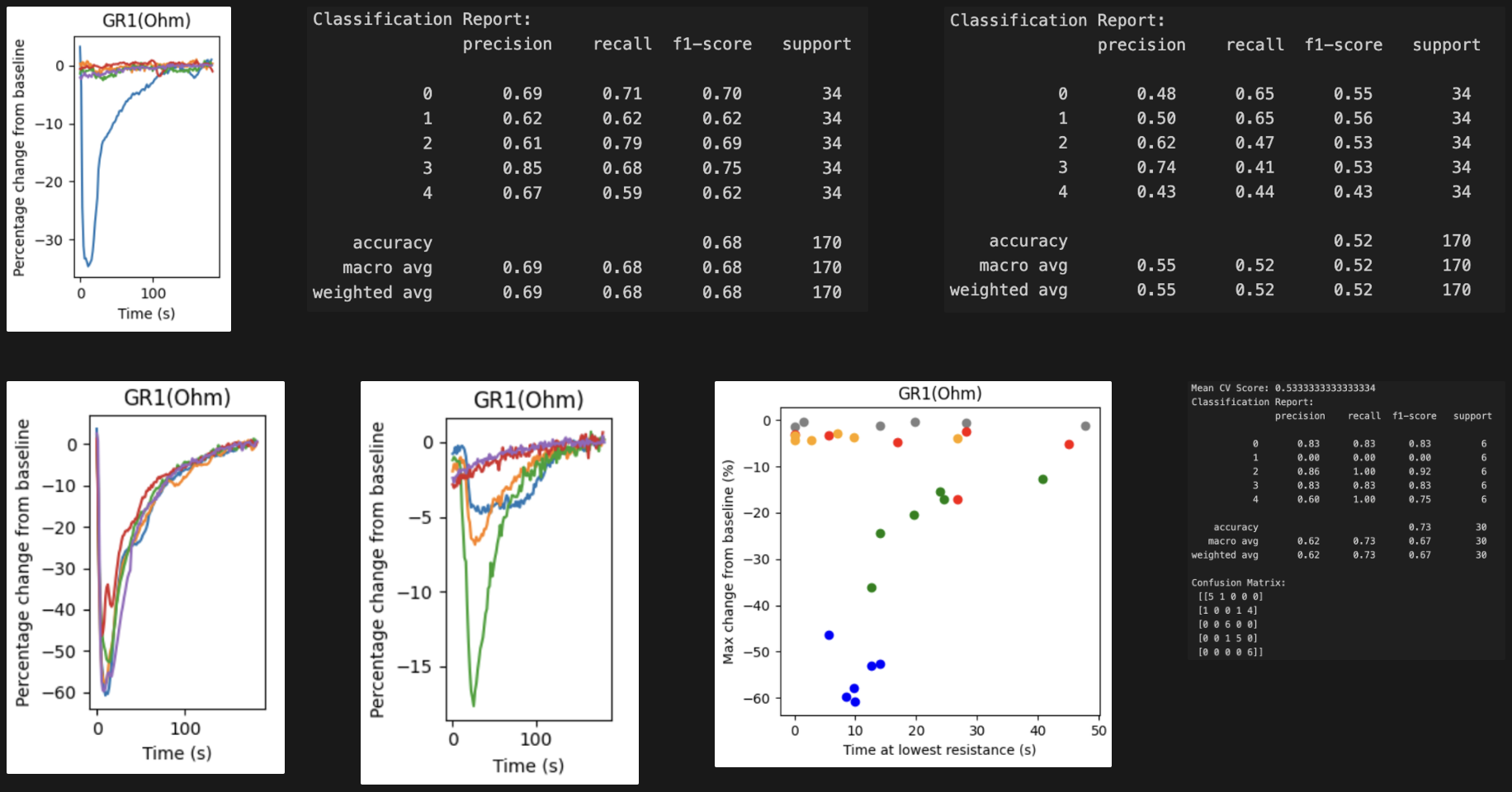
Figure 3: Sensor response to scents
- We also failed to observe any meaningful pattern in frequency when applying Fast Fourier Transform to the signal, as there is some variability across sessions.
- It became obvious that the classification will not be effective using linear increase in temperature for heater profile.
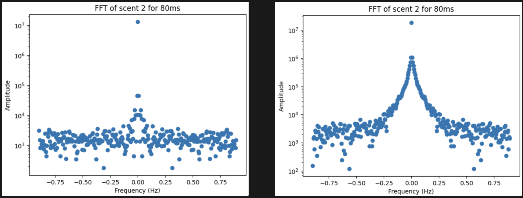
Figure 4: Fast Fourier Transform
- As linear increase in heater temperature yielded no promise, we used the default heater profiles in a variant of the sensor we use, BME688, which has multiple lab tested heater profiles for different applications. Our sensor differs with the 688 in that they have an array of 8 sensors, with a maximum of 4 heater profile configurations allowed for each measurement cycle, while we have exactly 1 sensor and a heater profile.
- We experiment with the default heater profile recommended by Bosch for general use cases, seen in figure 5.
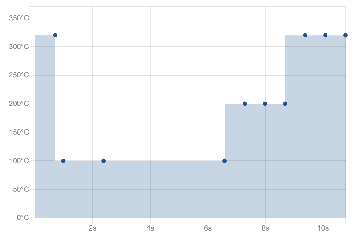
Figure 5: Bosch Recommended Heater Profile
- With the new heater profile, we hoped to observe more distinctive reaction patterns between different scents. The raw resistance readings were not immediately distinguishable between scents (figure 6).
- However, when using the last few measurement cycles of the stabilisation period as baseline to apply correction, it can be seen that scent 2 - 4 has a fairly distinguishable sensor reaction (figure 7).
- Scent 1 still suffers from the lack of reaction when compared to scent 0 (air), which means it received little to no reaction during emission.
- This is particularly intriguing, as scent 1 is peppermint, which is the most pungent scent of our testing group.
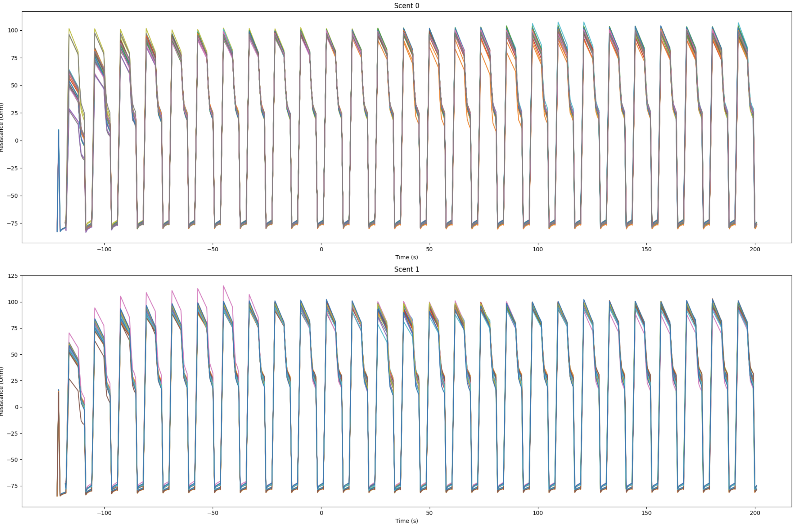
Figure 6: Raw Readings
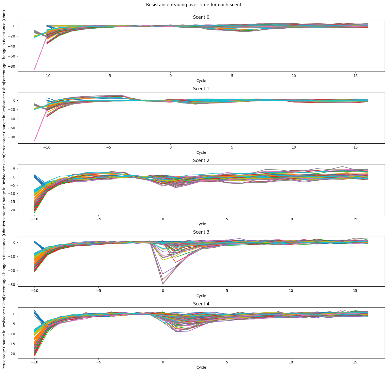
Figure 7: Baseline Corrected
- We extracted 4 features: (standard deviation and mean of resistance, percentage decrease in resistance and time at the lowest resistance) for each heater index, hoping that the sensor registers different reaction at different heater temperature between scents. However, upon visualisation of the features, it can be seen that the scent are not very distinguishable.
- With the KNN performing only marginally better than linear increase heater profile, we decided to separate the task into two phases, first establishing a robust classification algorithm in a more restricted environment, then transfer that to an open environment.
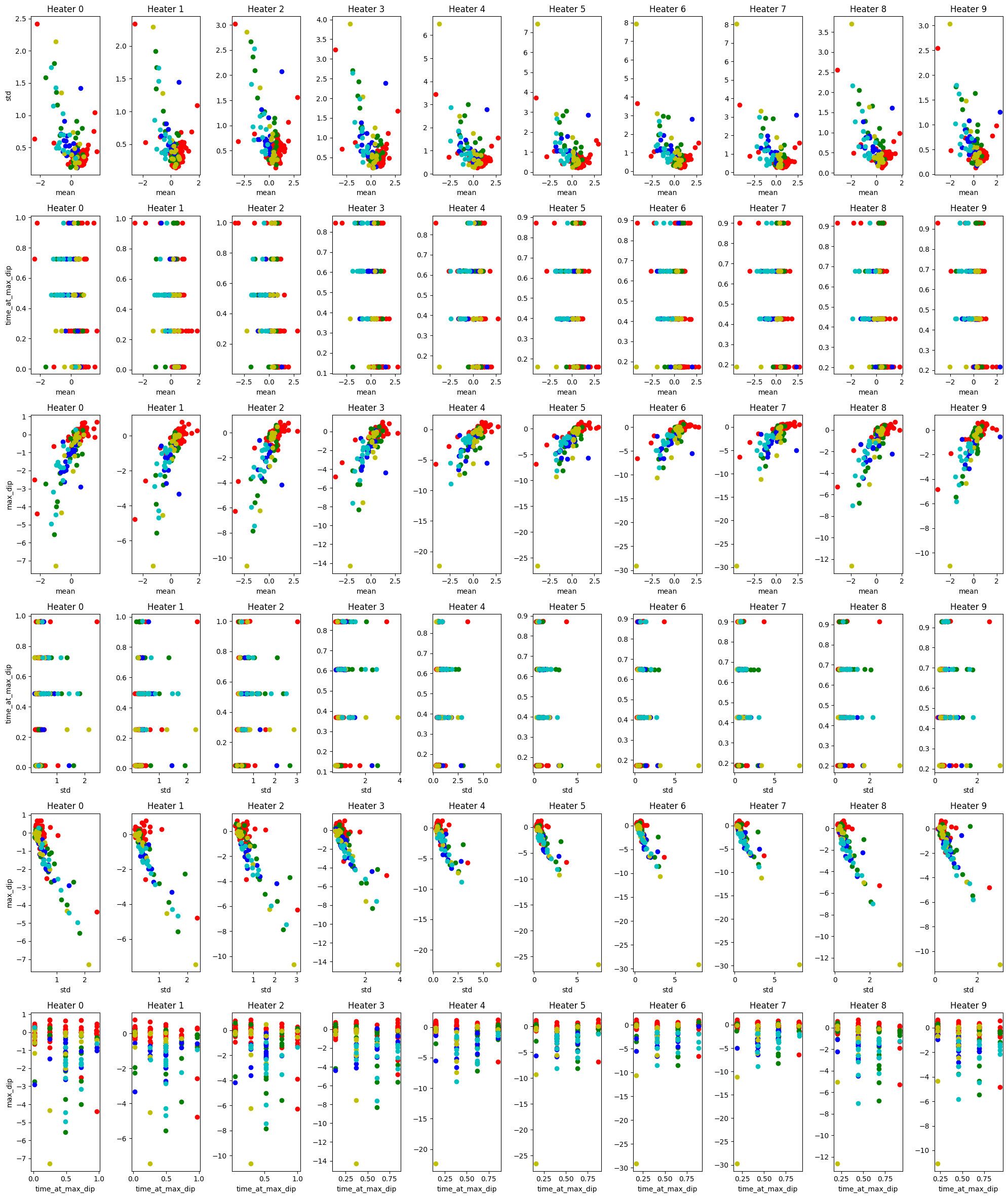
Figure 8: Visualising seperability of hand crafted features
- We move the data collection system in a large plastic container to see if the scents are not distinguishable, or if the concentration in an opened environment is insufficient for a single sensor to classify in open air.
- However, this setup introduces the issue of container contamination, as 50 regular emissions of 10 seconds for every scent may affect the reading we receive.
- We attempt to minimize this issue by leaving the container to dissipate the scent for 1.5 hours between scents.
- The baseline corrected results indicate that the container causes the scents to be vastly more distinguishable, even for previously dormant scent 1.
- It can be seen that the magnitude and swiftness of resistance decrease, and the rate of recovery in resistance greatly varies between scents.
- However, we also observe that the magnitude of response decreases as more samples are collected. We suspect this is due to insufficient time between scent emissions for dissipation.
- When using the same features as we did before, the scents are now much more distinguishable when visualized.
- We see the KNN performance massively increases with a closed container, when using the same features as the previous experiment, with accuracy consistently staying above 95%.
- We also trained a small ANN multi-class classification model to see if there are representations which can learned which cannot be seen with KNN. Results show an ANN increases the accuracy by 2-3%.
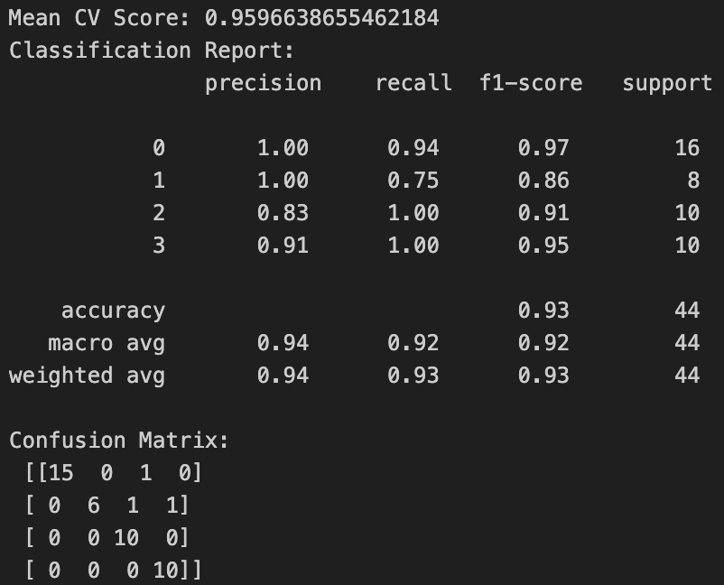
Figure 9: KNN with mean and standard deviation of resistance readings, as well as percentage decrease and time as minimum resistance..
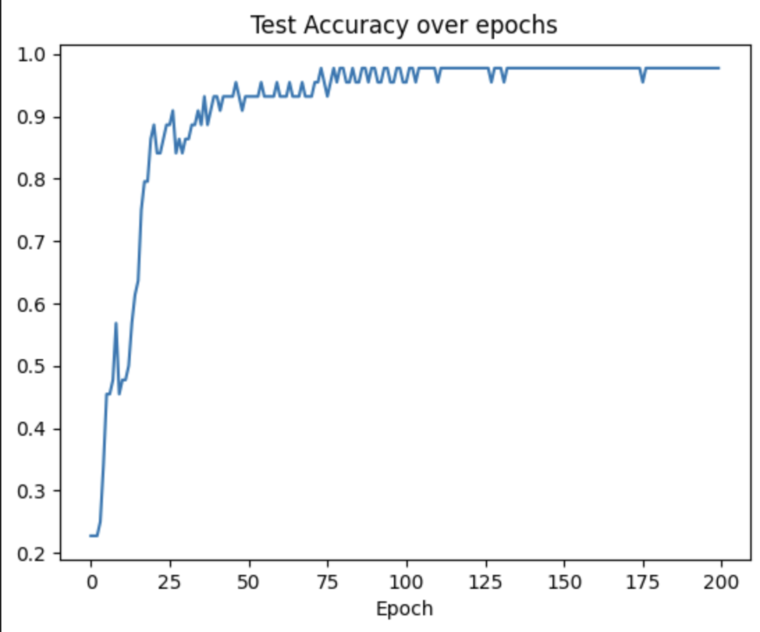
Figure 10: Test accuracy of ANN
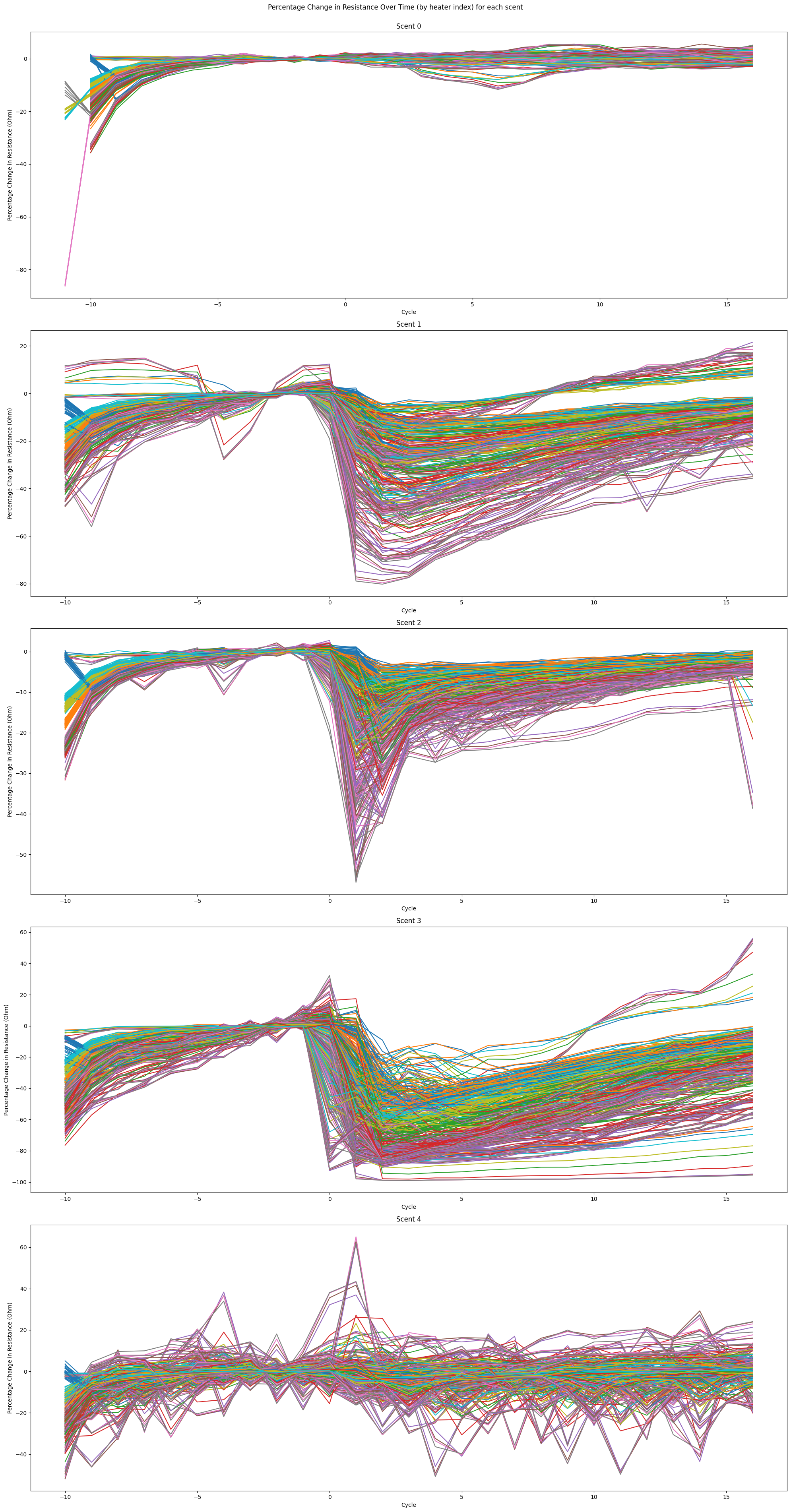
Figure 11: Resistance change over time for each heater index for each scent
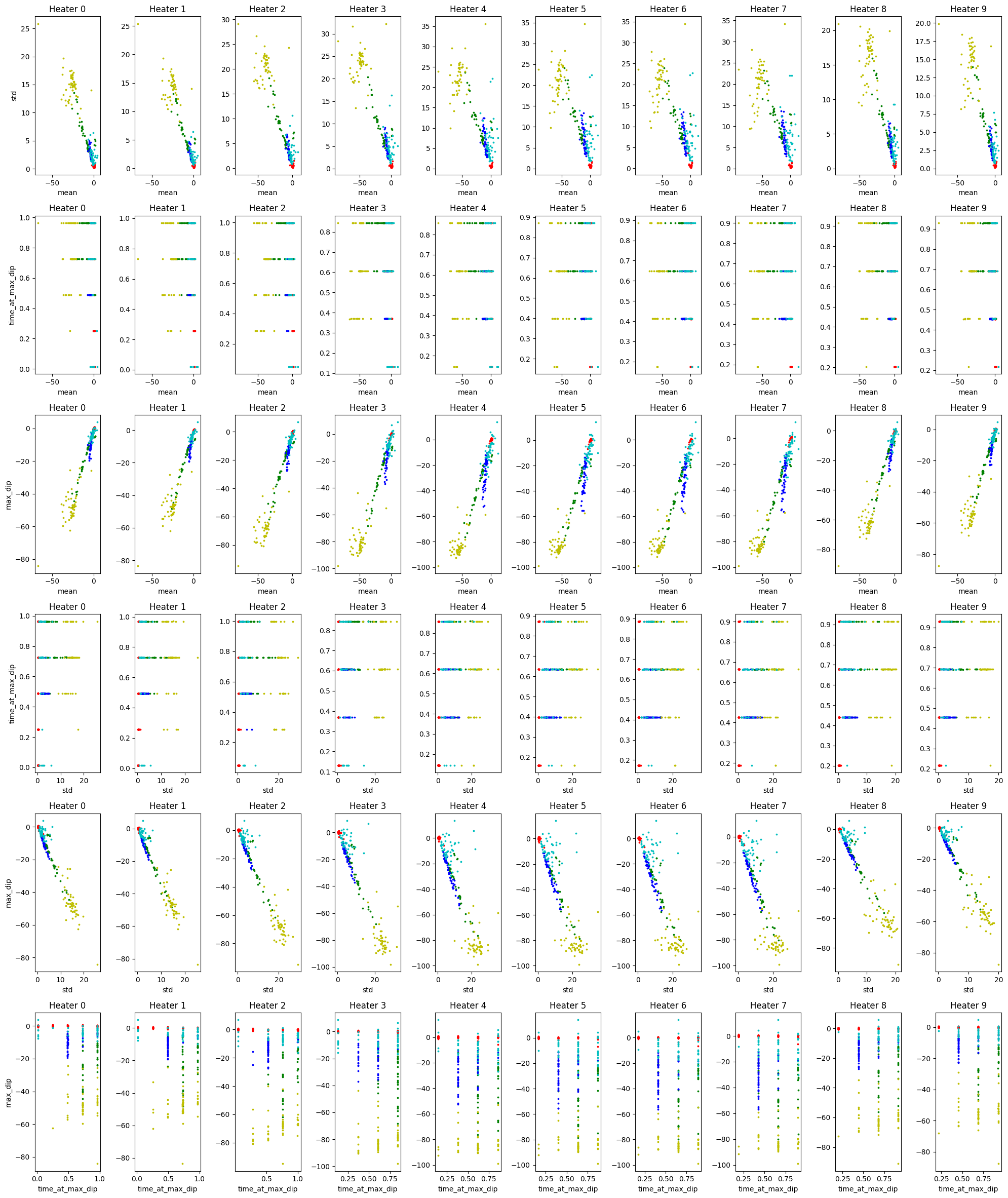
Figure 12: Visualising separability of hand crafted features
- Observing that scent 4 has fairly peculiar readings with high noise, we wanted to establish whether that is due to container contamination towards the end of the experiment (20+ hours)
- Hence, we repeated the experiment again but reversed the order to collect scent 0, then 4 to 1. We observe that the noise that not seen in the previous experiment become more prominent in scent 1 and 2, thus it is reasonable to say that the data collection can be heavily affected if there is contamination.
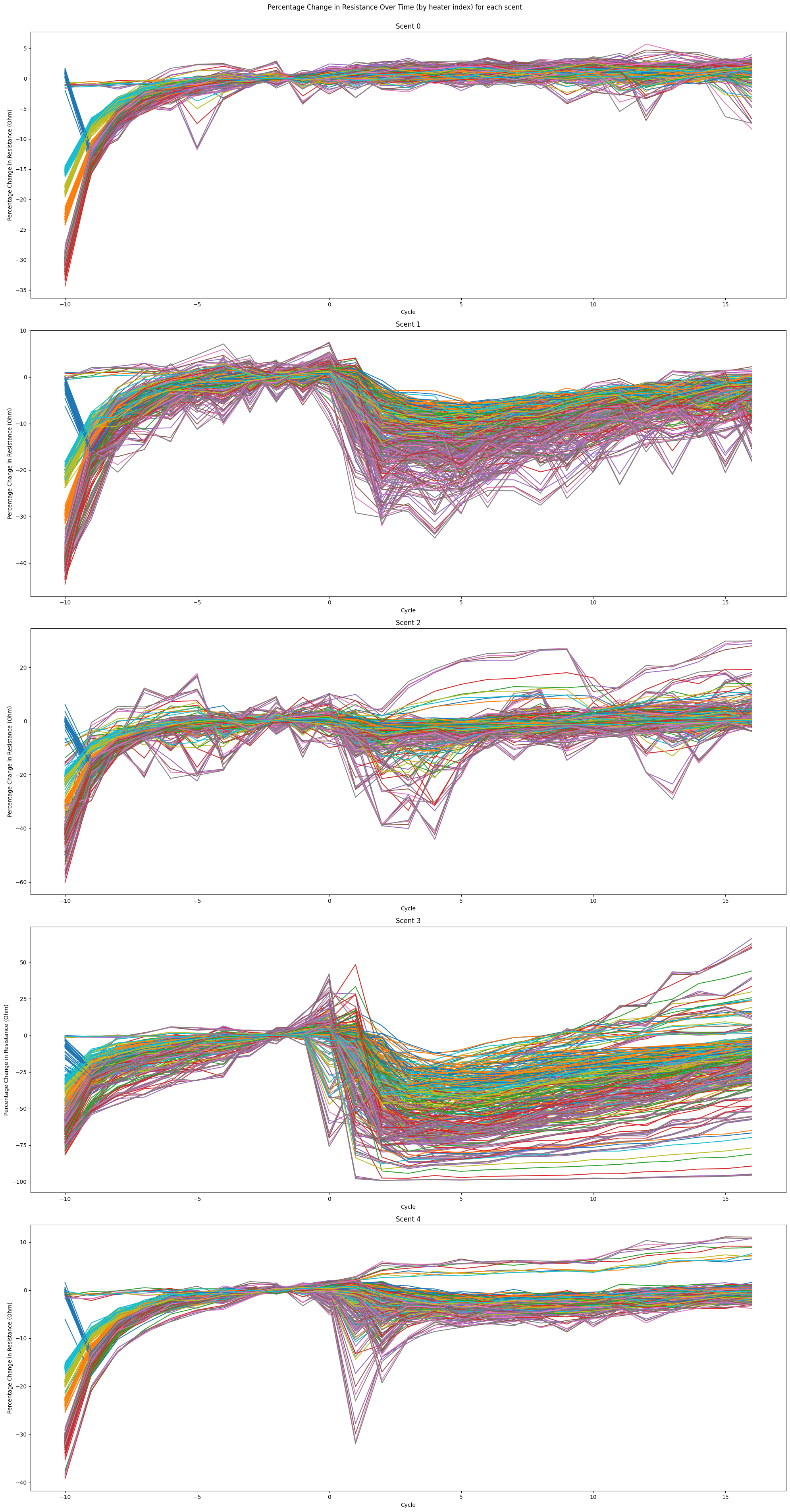
Figure 13: Reversed experiment observations
- To truly achieve generally applicable scent classification, we used automated feature extraction offered by the Python Library TsFresh, which forgoes the labor intensive hand crafted features, which are often only applicable to very narrow use cases.
- We use only standardisation in preprocessing so that sensor and session variability is minimised, so that the model is more generalisable.
- Once again we use a large plastic container around the setup to observe the performance difference between open and contained environments.
- We extract 658 features after the module auto-rejects irrelevant features.
- Using a simple MLP with the architecture below, we achieve a maximum of 97.89% accuracy.
- This shows around 2-3% improvement when compared to the previous experiments without automised feature extraction using the datasets collected in containers.
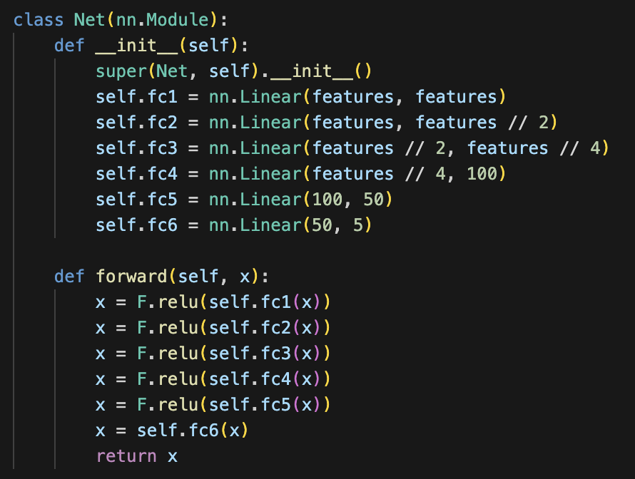
Figure 14: MLP Architecture
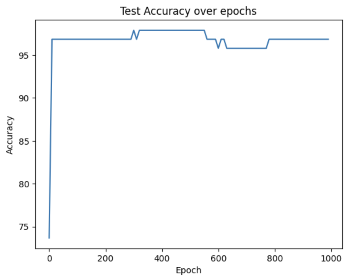
Figure 15: MLP Test Accuracy
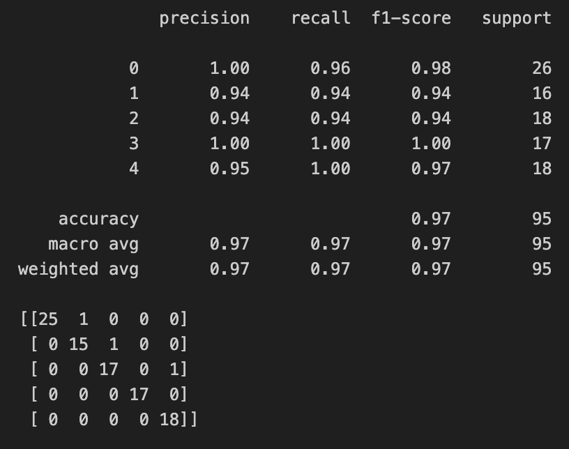
Figure 16: MLP Confusion Matrix
- It can be observed that out of 658 features, there are only 85 which are relevant to all 5 scent classes (p-value < 0.05).
- Hence, we train a smaller neural network to see these 85 features are adequate for classification tasks.
- We achieve 96.84% accuracy, indicating that the additional features provide marginal improvement to test accuracy. This implies the model can be miniaturised for training on hardware with limited compute such as Raspberry Pi.
- We observe that both confusion matrices have a sample wrong for air and for scent 1. Upon repeating the experiment, the confusion matrix is identical. This may indicate some samples, even when collected in the same session, can be hard to distinguish due to environmental factors and the variability of a single sensor.
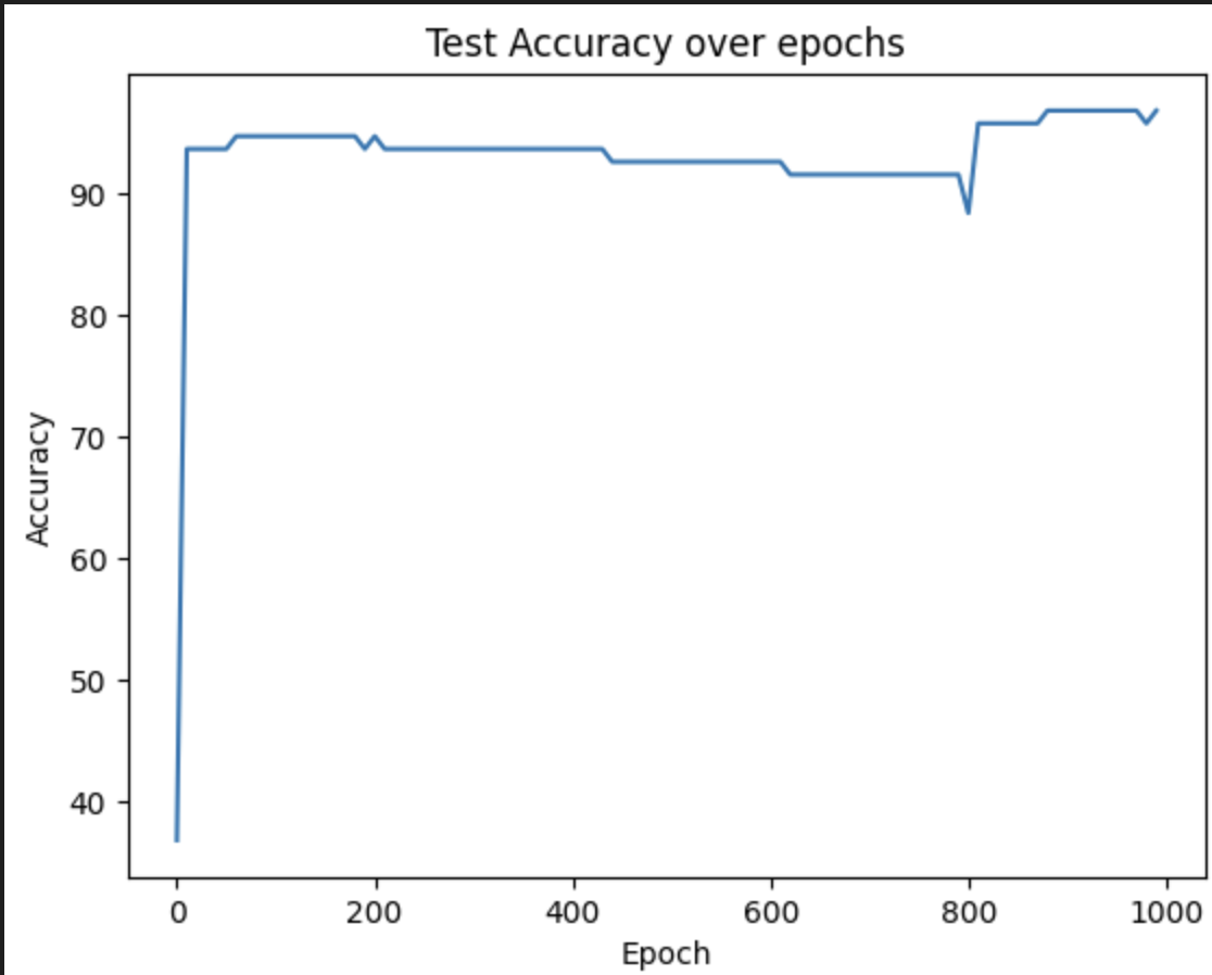
Figure 17: Test accuracy when training with 85 features
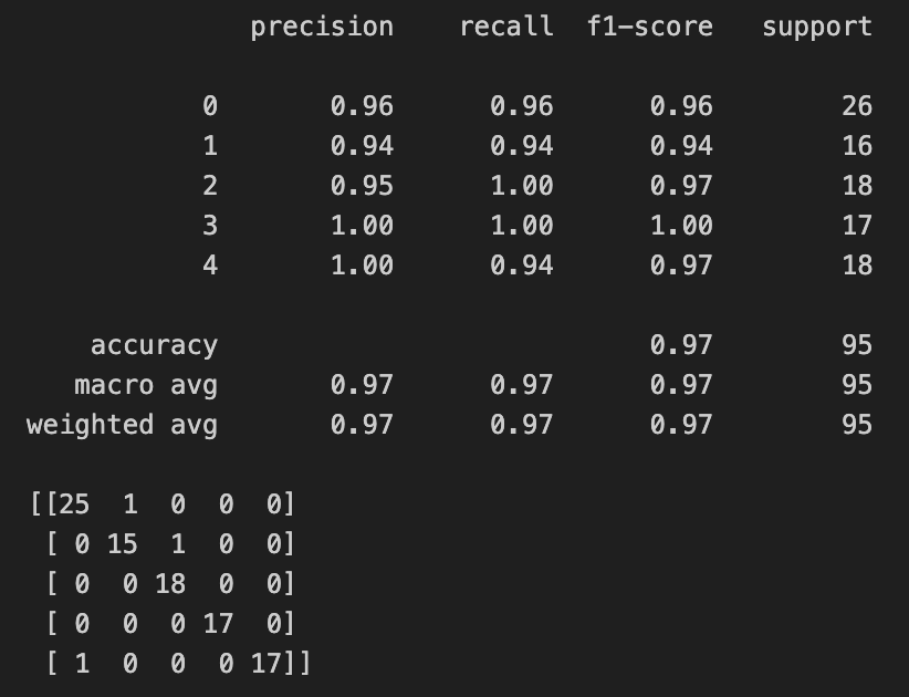
Figure 18: Confusion matrix when training with 85 features
- We investigate if the performance in contained environment can be sustained with data collected without a container, which is less prone to contamination but has seen less sensor reaction from the scent exposure in previous experiments, with higher variability.
- We extracted 204 features, and used this to train the same neural network as above, with a highest accuracy of 83.87%.
- This is a substantial improvement from the initial 70% we achieved with minimal feature extraction (and without).
- The feature relevance calculations show that no feature is relevant for all 5 scent classes, which differs from the contained experiment. This indicates the necessity for using more features when training a model for classification in open air to maintain acceptable performance.
- As TsFresh is primarily a time series feature extraction package, we wanted to avoid involving timestamps, which restricts the prediction frequency to the duration of scent emission cycle (3 mins), hence we discarded timestamps in favor of fixing a sample as a window of fixed number of heater cycles.
- This way, we force the model to learn the underlying representation without learning when a scent was emitted.
- We use 5 data points (5 heater profile cycles) as a sample. Each sample is about 50 seconds data.
- Each window takes approximately 1.5s for features extraction, hence makes it feasible for real time prediction of the scent.
- We retain 324 features of the original 783.
- Using the same neural network architecture as before, we achieve 79.8% accuracy on the test set, up from 70% when using manual and no feature extraction, but down from 84% from taking the entire measurement cycle as a window.
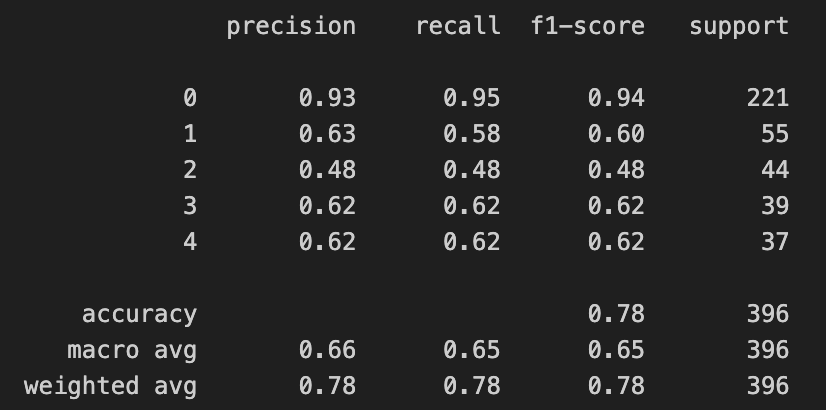
Figure 19: Confusion matrix of training with all classes of scents
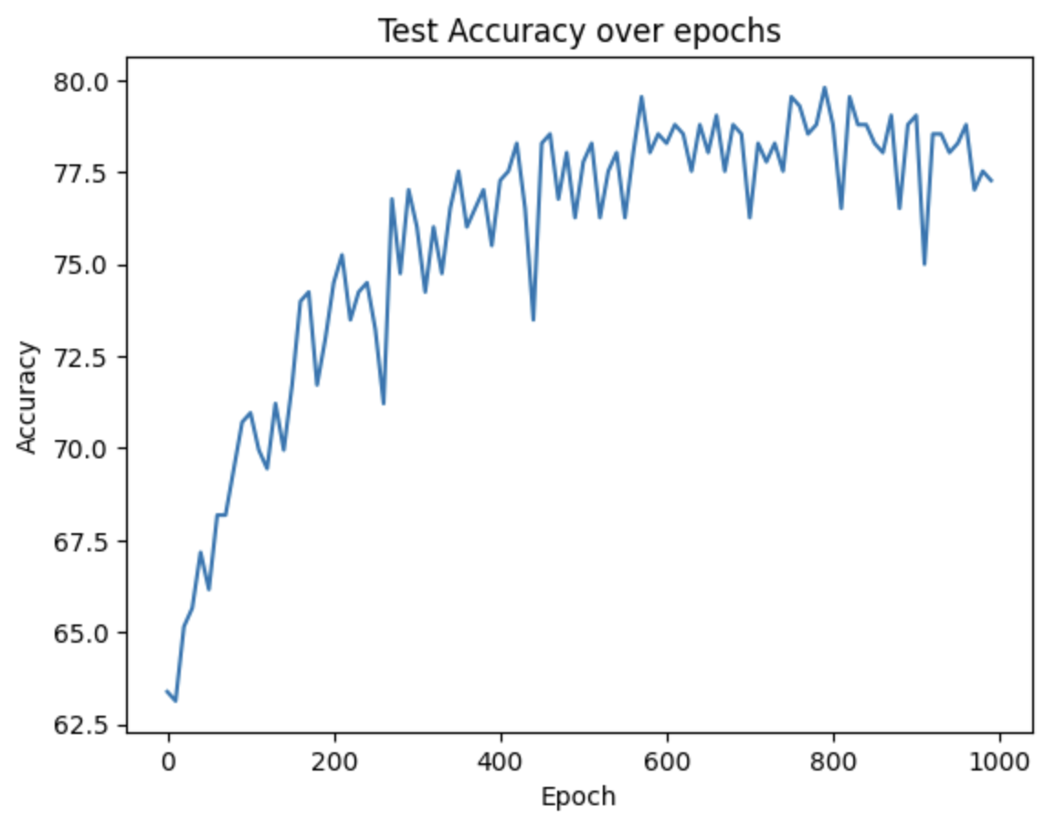
Figure 20: Using all 5 scents
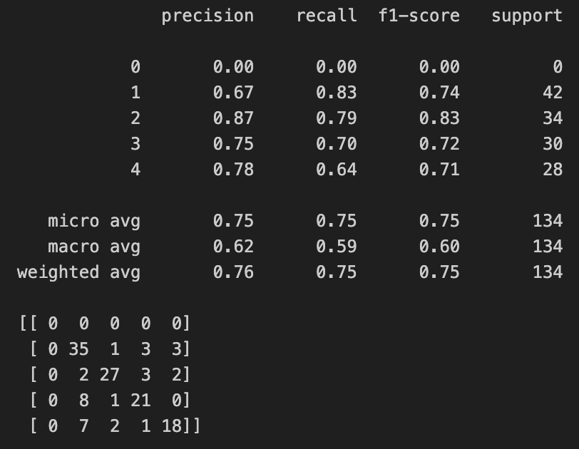
Figure 21: Results when excluding air (scent 0)
- Calculating the feature relevance as before, we retain 32 features that are relevant to the classification of all scents, which was not the case with the open environment without sliding window (which retained 0).
- Training on the 32 features that are relevant to the classification of all scents, we once again get 78.54% accuracy on the test set.
- To minimize class imbalance, excluding air from the dataset we get 76.12% accuracy.
-
We conclude that optimal time window is 7 heater cycles (~70s) without overlap (window with stride of 7 heater cycles), balancing prediction's temporal resolution with accuracy without overfitting.
- Smaller windows such as 5 seconds saw few percentages of decrease in accuracy.
- Results from our preceding experiments that show a simple ANN can deliver good test accuracy for classification tasks.
- ANN also shows the ability to learn underlying representations better than KNN.
- As the feature relevance is often varied between the scent classes in the dataset, the choice of n_significant, that is the threshold number of classes that a feature is relevant to (in a classification task), also varies depending on the specific task. Hence, we define a general block consisting of two fully connected linear layers with batch normalisation and dropout in between to reduce overfitting, and use ReLU for activation.
- The exact number of blocks (depth) and hidden dimension can then be defined depending on the number of features used for training, which may vary from task to task.
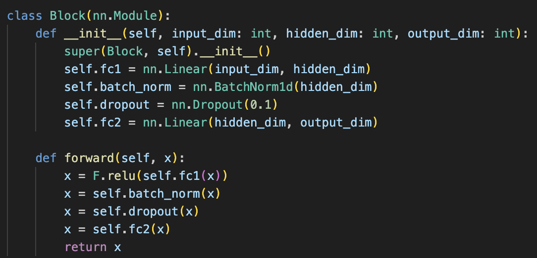
Figure 22: Final Machine Learning Architecture
- Initially, we had decided to go with the ESP32 as the brains of our system, as it was a lightweight, cheap and versatile microcontroller. It worked perfectly with the olfactometer and sensor, integrating the two.
- However, we soon realised that the processor on the ESP32 wouldn't be able to simulataneously run all the requirements for our project, so we decided to go with the Raspberry Pi.
- The Raspberry Pi was chosen due to its superior performance capabilities compared to the ESP32. Given the requirement to host a web server, run machine learning algorithms, and operate the olfactometer and sensor simultaneously, the Raspberry Pi offered the necessary computational power to handle these tasks efficiently.
- Unlike the ESP32, which required the olfactometer to be connected to a laptop, the Raspberry Pi facilitated standalone operation. This eliminated the need for constant user presence during operation, enhancing convenience and usability.
- Further, the Raspberry Pi's compatibility with Python was a significant factor in our decision-making process. Python's versatility and extensive libraries allowed for seamless integration of machine learning algorithms with the rest of our project components. This streamlined development and facilitated efficient communication between different parts of the system.
- The Raspberry Pi also benefits from a robust ecosystem of community support, documentation, and resources. This ensured accessibility to troubleshooting guides, tutorials, and libraries, simplifying development and troubleshooting processes.
- The Raspberry Pi's scalability made it well-suited for potential future expansions or modifications to our project. Its ability to handle additional sensors, peripherals, or functionalities provided flexibility for future enhancements or iterations of the system.
- [1]R. Gosangi and R. Gutierrez-Osuna, “Active temperature modulation of metal-oxide sensors for quantitative analysis of gas mixtures,”Sensors and Actuators B: Chemical, vol. 185, pp. 201-210, Aug. 2013, doi: https://doi.org/10.1016/j.snb.2013.04.056.
- [2]J. Palacín, E. Rubies, E. Clotet, and D. Martínez, “Classification of Two Volatiles Using an eNose Composed by an Array of 16 Single-Type Miniature Micro-Machined Metal-Oxide Gas Sensors,”Sensors, vol. 22, no. 3, p. 1120, Feb. 2022, doi: https://doi.org/10.3390/s22031120.
- [3]H. Liu, R.-J. Wu, Q. Guo, Z. Hua, and Y. Wu, “Electronic Nose Based on Temperature Modulation of MOX Sensors for Recognition of Excessive Methanol in Liquors,” vol. 6, no. 45, pp. 30598-30606, Nov. 2021, doi: https://doi.org/10.1021/acsomega.1c04350.