MODEL DESCRIPTION
For our Object Detection model we decided on using Google’s TensorFlow Object Detection API (Link). Within the repository, there are already few preset detection models to choose from. Although it would be possible to design our own model, we felt that given the time constraints, it would be unlikely to produce a model with significant performance improvements to the ones given. This is especially true considering these models have been trained and tested thoroughly given that this software is being used by such a renowned company as Google.
When picking a model, two models stuck out in particular to us. These two models were ssd_mobilenet and faster_rcnn, the later giving better precision but slightly slower speeds. Due to the conditions in which our application would be used, we decided to use the faster_rcnn model. The live video will mostly be stationary will several objects that may look similar in view. Therefore, we are more concerned about precision in the detection, and less about the speed. However the speed still had to be sufficient to analyze a video feed at a fast rate.
UNIT & INTEGRATION TESTING
To train the model we used the train.py script that is currently located in the legacy folder of the repository. We downloaded the faster_rcnn_inception_v2_coco model, found in the ‘TensorFlow detection model zoo’ section of their repository, and trained it using our own images of medical instruments. We used the faster_rcnn_inception_v2_coco.config file provided and didn’t alter any of the hyper-parameters except the for the ones needed to change the training pipeline (train and test file paths, number of classes e.t.c).
With our latest version of the model, we trained the model on 3 different instruments categories (forceps_straight, forceps_curved and tweezers). For each category, we only used 1 specific instrument to take our images as we were very limited to the number of instruments we had available to us. In total we took around 1500 images of the instruments with a pretty equal distribution between the different categories. The images consisted of a mixture of single and multiple instruments within the shot. They were taken in a wide variety of backgrounds, lighting and with a wide selection of different objects scattered around the image. After taking the images we then had to label all the instruments that we want the model to detect, we used labelImg to do this (Link). We also removed about 10% of the images selected randomly from the training pipeline which we will later be used testing. Using TensorBoard we could see the progress of our training by checking how the loss of the model changed while training. We stopped training the model when the total_loss plateaued for around half an hour, which averaged out to be around 0.05.
TESTING THE MODEL
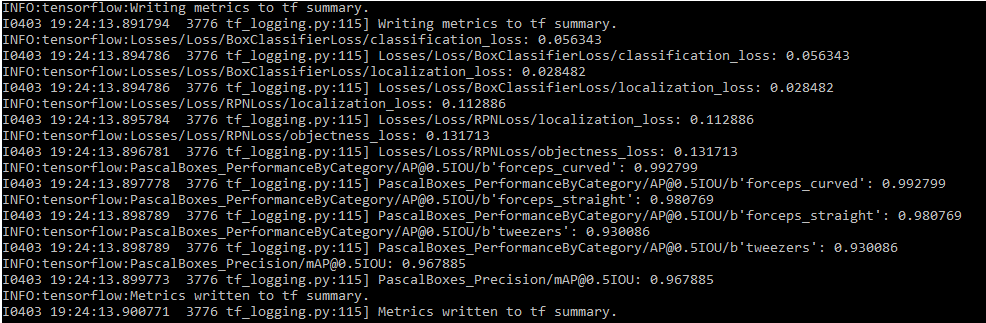
As mentioned earlier we removed around 10% of the images and put them into the testing pipeline. To get our first metric for the performance of our model, we ran the eval.py script that is currently located in the legacy folder of the repository. This script calculates the mean Average Precision (for more detail about mAP - Link) for each category and the model as a whole using the images in the test pipeline. Using those 10% of images, the script found the mAP to be around 0.97. The exact values can be found below.
The images in the testing pipeline are very similar to the ones used in the training set as they were directly taken from it. Therefore the mAP is not an accurate representation of the performance of the model in real life. Therefore to get a measurement of how the model would perform in our application we had needed to test the model on different images, ones that the model has not seen before. We also wanted to take into consideration the environment in which the images would be taken. Therefore we used mainly plain backgrounds for our second batch of test images with different arrangements of bright lights to mimic a clinical environment.
For our project we could have trained our model a wide a set of categories as possible however, this would not really be beneficial given the time constraints. We wanted to test the performance that an object detection model would have on the two ends of the spectrum of classifying medical instruments. Therefore, we selected 2 instruments which looked very ‘similar’ (forceps_straight, forceps_curved) and 2 instruments that looked very ‘different’ (forceps_straight, tweezers) to train our model on, allowing us to compare the performances. For our testing images, we also created two sets of images. One for comparing the 2 ‘similar’ instruments and the other for for the ‘different’ instruments. For each set we took 35 images, containing 50 objects to be detected. The breakdown of how we took the images can be seen here:
2 different white backgrounds in different lighting conditions:
Single object photos (For each - 20 total):
6 no flash
4 with flash
Double object photos (15 total):
6 no flash
7 with flash
2 on wooden surface (1 with flash, 1 without)
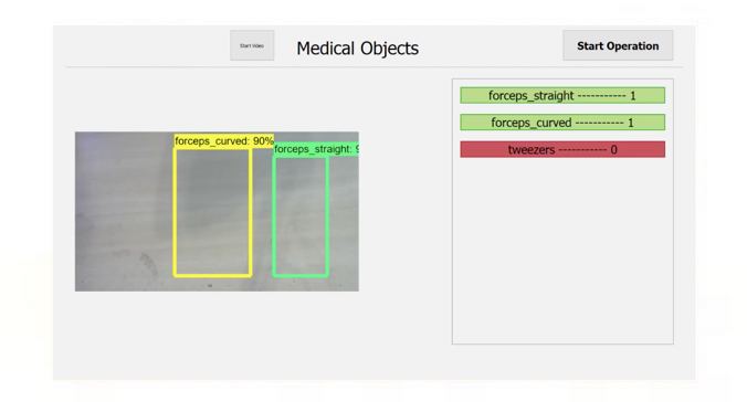
After taking the images we ran the two sets through our model to get the predictions. From the data, we only took into consideration objects with a 75% accuracy or above. All the results can be found here (Link) with the images separated into 2 folders for the 2 sets (only shows top 5 detections for each image). The summary of my evaluation can be found in the “Detection data evaluation.xlsx” file in the folder. If there were multiple boxes around an object, it would be classified into the category with highest accuracy. Our application does not currently check for boxes over the same object. Therefore this would cause 2 objects to come up in the list if this occurs. This is because we assume a ‘perfect’ model and therefore each object would be labeled with 1 category. However, if we could work on the application further we would make it only show the largest accuracy label for each object.
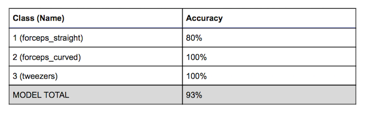
The result for both sets were very quite similar. The only wrong predictions in the tests involved trying to guess instrument class 1 which was in both sets. The other item in both sets had an accuracy of 100%. Furthermore, all the wrong predictions involved falsely identifying instrument 1 with instrument 2. Also all the extra detections of an object involved predicting either instrument 1 or 2 as the other. This was to be expected as the instruments 1 and 2 were the ‘similar’ objects and they were also very hard for us to distinguish by eye from a picture too. From our tests we got the following accuracies for each class and the whole model which was just an average of all the classes:
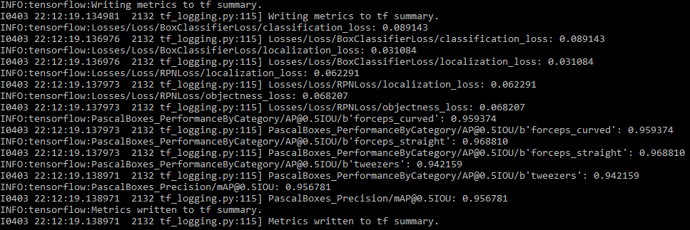
We also passed the images of both sets through the eval.py to calculate the mAP on those images and we got these results:
EVALUATING RESULTS AND CONCLUSIONS
After evaluating the model using mAP on more realistic images we got a mAP of 0.956 which is lower than the evaluation on the 10% set of images. This is to be as expected however it is still very high. From these numbers we can say that our model can distinguish between the instruments quite accurately at our current stage of the project.
After investigating into the individual images and the detections along with them in more detail, we can produce more deductions about our model. We can say our model can differentiate very different looking medical instruments with near 100% accuracy in a wide variety of settings. This is because all the errors in the tests for ‘different’ set were caused by by the ‘similar’ set of instruments.
Although the model can distinguish the ‘similar’ objects with still quite a high accuracy (around 90%), there are a lot of side effects caused by training on such instruments. Sometimes the model puts both categories over the instrument, which for our application causes it to think there is an extra instrument in the image. Although this can be gotten around by adding a filter to the data, there are still a lot of problems which can cause inaccuracies in our data.
The images we took for testing were still images and of reasonable resolution. Our testing assumes the objects in the images are in a condition which they can be distinguishable. However, in a live feed, the images may be of lower resolution and can be a bit blurry due to the movement of the instruments. Thus lowering the accuracy of the model significantly as there is no guarantee that the ‘similar’ instruments are in a state that they can be distinguished. Even assuming a ‘perfect’ model, one in which it only puts each instrument in only 1 category at a 90%+ accuracy (percentage of times it can label such instruments in each category), the application still depends on the quality of the images being fed into the input. While, the resolution of the video feed can be increased, this would cause a reduction in responsiveness as it would take longer to analyze each frame.
To conclude, by testing the limits of Computer Visions technology we have found that they have the capabilities to distinguish very similar looking medical instruments. However when using such technologies for live video, the accuracy of the model has to be much larger to produce a reliable output. Therefore, the range of categories or how specific you would like to classify an instrument has to be limited. The model should be thoroughly on whether it can reliable distinguish the instruments in which you train them on before being distributed. As, external factors such as image quality will affect the performance of the model in the use of our application.