Algorithm
Algorithm and Experimentation
Table of Contents
Vector Similarity Check
In-depth Analysis of Similarity Measures
Cosine Similarity
The cosine similarity metric assesses the cosine of the angle between two non-zero vectors in an inner product space. It is a measure of orientation and not magnitude, with two vectors with the same orientation having a cosine similarity of 1, and vectors at 90° having a similarity of 0. The mathematical representation is:
cos(θ) = \(\frac{A \cdot B}{\|A\|\|B\|}\)
Where \(A\) and \(B\) are two non-zero vectors, \(A \cdot B\) denotes their dot product, and \(\|A\|\) and \(\|B\|\) are the Euclidean norms of \(A\) and \(B\) respectively.
Euclidean Distance
The Euclidean distance (or Euclidean norm) is the "straight-line" distance between two points in Euclidean space. This is the root of the sum of the squares of differences between individual elements of two vectors. Its formula is:
d(A, B) = \(\sqrt{\sum_{i=1}^{n} (A_i - B_i)^2}\)
Where \(A\) and \(B\) are two vectors and \(A_i\) and \(B_i\) are their respective \(i^{th}\) elements. This measure can become problematic in high-dimensional spaces where all points tend to be equidistant from each other, a phenomenon known as the curse of dimensionality.
Manhattan Distance
The Manhattan distance is the sum of the absolute differences of their coordinates, often used in geometry as the distance between points on a grid (based on paths parallel to the axes). Mathematically, it is given by:
D(A,B) = \(\sum_{i=1}^{n} |A_i - B_i|\)
Where \(A\) and \(B\) are two vectors and \(|A_i - B_i|\) is the absolute difference between their respective \(i^{th}\) elements. In the context of high-dimensional vector spaces, this distance metric can be more informative than the Euclidean distance, as it measures the distance traversed to get from one data point to another.
Theoretical Underpinnings of Word Embeddings
Word Embeddings and Semantic Space
Word embeddings are a class of approaches for representing words and documents using a dense vector representation. They are an essential step in representing language data to machine learning algorithms. When we train a model to embed words, we are essentially training it to reduce the dimensionality of the text data, such that the resulting vectors capture some semantics of the words based on the distances and directions from one another. These models map semantic meaning into a geometric space, often referred to as a semantic space. This space is usually of much lower dimensionality than the space of all possible words, where each dimension captures some aspect of the word's meaning and the distances between words in that space are related to the semantic distances between the words.
Utilizing Sentence Transformers for Embeddings
Sentence transformers like the all-MiniLM-L6-v2 are designed to convert sentences and words into high-dimensional space vectors. The transformer model does this by using the context around each word, thus capturing not just the word but the concept it represents in the context it's used. This allows us to perform arithmetic operations on the words, like finding the average to get sentence embeddings, or adding and subtracting vectors to find analogies. The embeddings thus obtained can then be used to compute the various similarity measures discussed above to identify words with similar contexts or meanings.
Detailed Experiment Procedure
The crux of the experiment lies in embedding words into a continuous vector space where semantically similar words are mapped to nearby points. The all-MiniLM-L6-v2 model is leveraged to create these embeddings. This model has been chosen due to its robust performance on various NLP tasks and efficiency in capturing the semantic nuances of language. With 'jump', 'punch', and 'speak' as anchor points, we explore their semantic field by mapping synonyms into the same space using vector representations obtained from the model. The k-means algorithm is then applied to cluster these points. The underlying assumption is that words closer in the vector space share closer semantic meanings.
K-Means Clustering: Theoretical Perspective
K-Means clustering is a partitioning method that segregates n observations into k clusters in which each observation belongs to the cluster with the nearest mean. The optimization problem at the core of K-Means clustering is to minimize the sum of the squared distances between each point and the centroid of its cluster. Mathematically, the objective function, known as inertia or within-cluster sum of squares (WCSS), is defined as:
\( J = \sum_{j=1}^{k} \sum_{i=1}^{n_j} \| \mathbf{x}_i^{(j)} - \boldsymbol{\mu}_j \|^2 \)
where \( n_j \) is the number of observations in the \( j^{th} \) cluster, \( \mathbf{x}_i^{(j)} \) is the \( i^{th} \) observation in the \( j^{th} \) cluster, and \( \boldsymbol{\mu}_j \) is the centroid of the \( j^{th} \) cluster.
The algorithm iterates through two main steps: (1) assignment of data points to clusters where each point is associated with the nearest centroid, and (2) update of centroids to the mean location of all the points in that cluster. These steps are repeated until the centroids stabilize, and the algorithm converges.
Comprehensive Evaluation and Discussion

Graphical and Cluster Analysis
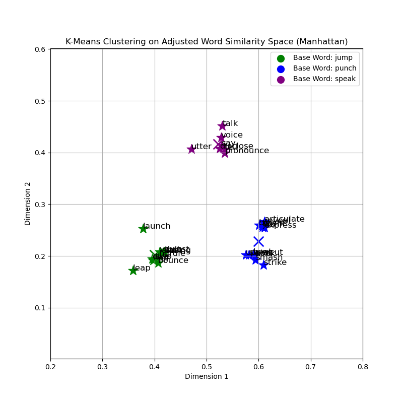
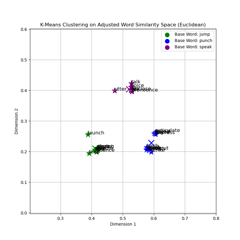
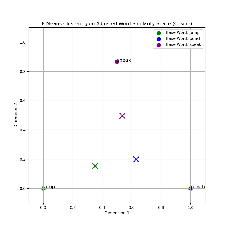
The provided graphs visualize the clusters of words obtained using the K-Means algorithm with different similarity measures. The clusters are color-coded based on the base words: 'jump', 'punch', and 'speak'. From the cosine similarity graph, the clusters around each base word appear cohesive, indicating that words with similar meanings are indeed closer in the vector space. This is an expected trend since cosine similarity evaluates the angle between vectors, effectively grouping words by their contextual relationship rather than by their magnitude difference.
In contrast, the Euclidean distance may produce less cohesive clusters, particularly in high-dimensional spaces where the distance between any two points becomes less meaningful due to the curse of dimensionality. This can lead to more dispersed clusters and potentially less accurate representations of the underlying semantic relationships.
A deeper comparative analysis reveals that cosine similarity, focusing on angle rather than magnitude, is inherently suited for the comparison of documents of different lengths and is less sensitive to the accumulation of irrelevant features. Euclidean and Manhattan distances, while straightforward in their computation, may not encapsulate the intricacies of semantic similarities as effectively in high-dimensional spaces such as those employed by word embeddings.
| Similarity Measure | Base Word: jump | Base Word: punch | Base Word: speak |
|---|---|---|---|
| Cosine Similarity | 0.3859 | 0.3724 | 0.4195 |
| Euclidean | 0.4624 | 0.6440 | 0.6277 |
| Manhattan | 0.4485 | 0.6460 | 0.6339 |
Interpretative Analysis
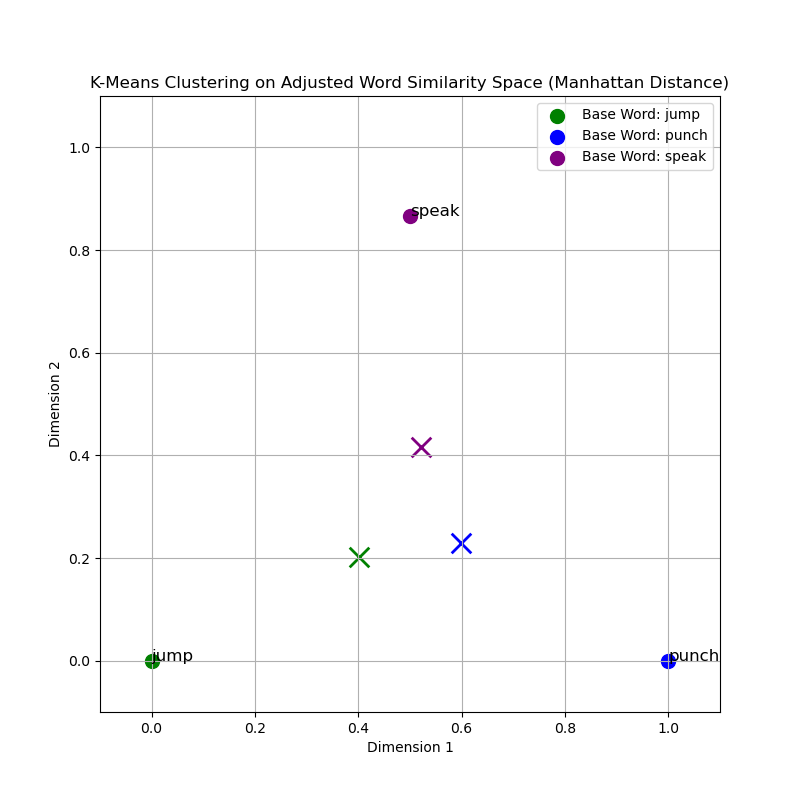
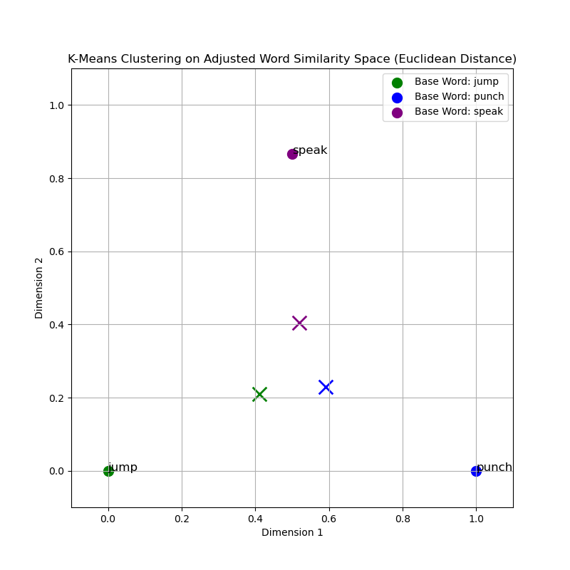
The distances between the base points and the cluster centroids reveal insights into the compactness and separation of clusters formed by different similarity measures. Cosine similarity, which accounts for the angle between vectors, typically forms tighter clusters for semantically related words. This is evident from the relatively smaller distances of centroids to the base points, signifying a more concentrated grouping around the conceptual epicenter represented by the base words.
In contrast, the Euclidean and Manhattan distances, which consider linear and block distances respectively, result in centroids that are farther from the base points. This suggests that when using Euclidean or Manhattan distances, the clusters have a larger spread in the vector space. The greater distances could also imply a less accurate capture of semantic relationships within the clusters.
Therefore, the Cosine similarity measure appears to provide a more meaningful clustering of words in a high-dimensional semantic space, resonating with the inherent nature of language where meaning is more about the relationship between words rather than their absolute positions.
Conversely, the Euclidean distance graph demonstrates a less defined clustering pattern, which could be attributed to the curse of dimensionality. In a high-dimensional space, such as that of word embeddings, the Euclidean measure may not perform as effectively due to all points tending to be equidistant from one another.
Evaluation and Selection of the Optimal Similarity Measure
In comparing the two graphs, it is clear that cosine similarity results in more distinct and semantically meaningful clusters. This measure aligns well with the distributional hypothesis in linguistics, which posits that words occurring within similar contexts tend to have similar meanings. For tasks requiring an understanding of semantic content, such as identifying synonyms or related terms, cosine similarity outperforms Euclidean distance.
Therefore, based on the analysis of the clustering patterns and inherent properties of the similarity measures, cosine similarity is the optimal choice for clustering words by semantic similarity in a high-dimensional embedding space.
When evaluating the effectiveness of cosine similarity versus Euclidean distance in the context of word embeddings, the former often proves to be superior. The cosine similarity focuses on the angle between vectors, thereby capturing the relational nuances in word meaning, regardless of vector magnitude. This characteristic is particularly advantageous when working with normalized vectors of word embeddings.
Model Efficiency and Accuracy Analysis
Exploration of NLP Model Efficiency
In our continuous effort to optimize performance and efficiency in natural language processing tasks, we explore various models to find the perfect balance between size, load time, and accuracy. Considering our client's requirements for a robust and compact model, we focus on evaluating models that are not only accurate but also have small file sizes and quick load times. I have already attempt to repeat the first experiment with all these model but the accuracy proof to be very similar so in a way it can be say that it insignificant and we should look more into the size of the model.
Comparative Analysis of NLP Models
Below is a comparative analysis of different models including the all-MiniLM-L6-v2 model that we have utilized. The table outlines key attributes such as model size and potential for fine-tuning, which are crucial for our application needs.
| Model | Size | Potential for Fine-tuning |
|---|---|---|
| all-MiniLM-L6-v2 | 80 MB | High |
| DistilBERT | 256 MB | Medium |
| MobileBERT | 100 MB | Medium |
Evaluation and Selection Criteria
The selection of the most appropriate model for our application is based on a comprehensive evaluation of several factors, including model size, load time, accuracy, and the potential for fine-tuning. Given the constraints of our application, which demands a robust and small model for faster loading times, the all-MiniLM-L6-v2 model emerges as a particularly suitable choice. Its relatively small size, combined with the high potential for fine-tuning, makes it an ideal candidate for our purposes.
Advantages of Fine-tuning
One significant advantage of opting for models like all-MiniLM-L6-v2 is their high adaptability through fine-tuning. By adding our own dataset, we can enhance the model's accuracy for our specific requirements without substantially increasing its memory footprint. This process allows us to tailor the model more closely to the nuanced needs of our application, providing a bespoke solution that maintains efficiency while improving performance.
In conclusion, the all-MiniLM-L6-v2 model offers an optimal balance of efficiency, speed, and accuracy for our needs. It stands out as the most suitable option for applications requiring high performance in a compact form factor. Further, its high potential for fine-tuning ensures that we can achieve even greater accuracy tailored to our specific use case, making it the ideal choice for our project.
Understanding NER Model Training
Algorithmic Deep Dive into NER Model Training
The NER model training algorithm optimizes the model parameters through an iterative process, adjusting the internal state of the model to minimize prediction errors on the training data. This process involves backpropagation and stochastic gradient descent (or a variant thereof) as fundamental mechanisms for learning.
Mathematical Foundation: The NER training can be mathematically characterized by an objective function, often a loss function such as cross-entropy, which quantifies the difference between the predicted and actual classifications for the training examples.
Cross-Entropy Loss Function:
\( L(\theta) = -\frac{1}{N} \sum_{i=1}^{N} \sum_{c=1}^{C} y_{ic} \cdot \log(p_{ic}(\theta)) \)
where \( N \) is the number of training examples, \( C \) is the number of entity classes, \( y_{ic} \) is a binary indicator of whether class label \( c \) is the correct classification for observation \( i \), and \( p_{ic}(\theta) \) is the predicted probability that observation \( i \) belongs to class \( c \) given the model parameters \( \theta \).
Gradient Descent: The optimizer modifies the parameters \( \theta \) in the direction of the negative gradient of the loss function with respect to those parameters. The update rule is given by:
\( \theta_{\text{new}} = \theta_{\text{old}} - \alpha \nabla_\theta L(\theta) \)
where \( \alpha \) is the learning rate, and \( \nabla_\theta L(\theta) \) is the gradient of the loss function with respect to \( \theta \).
Rationale for Approach: This iterative optimization is necessary because NER is a complex function approximation problem. By iteratively updating the model, we ensure that the most informative features for predicting entity classes are encoded within the model's parameters, enabling the recognition of entities in varied linguistic contexts.
Additionally, regularization techniques may be applied to prevent overfitting, and techniques like dropout are used during training to improve the model's generalization ability. The use of a dropout rate (in the update function, denoted as 'drop=0.5' in the code) randomly zeroes a subset of outputs from neurons, which helps in simulating the training of multiple neural network architectures and encourages the model to develop more robust features.
The iterative training with shuffled data (to prevent the model from learning patterns specific to the order of examples) and the progressive monitoring of loss values are crucial for diagnosing the training process. They allow for the early detection of issues such as underfitting or overfitting, and for the adjustment of hyperparameters to refine the model's learning trajectory.
Training Loss Interpretation
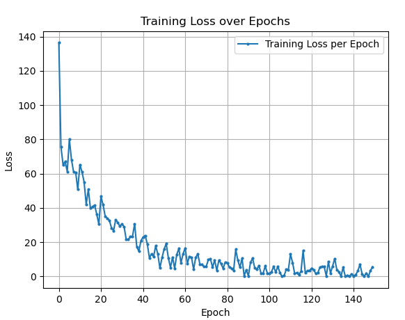
The graph presents a typical descent in loss value as the number of training epochs increases. Initially, there is a sharp decline in loss, indicating that the model is rapidly learning from the training data. The substantial decrease at the start suggests that the model's initial parameters were far from optimal and that early iterations brought significant improvements.
As training progresses, the rate of loss reduction slows down, and the curve begins to flatten. This deceleration is expected and denotes that the model is starting to converge to a set of parameters that minimizes the loss function. It reflects the diminishing returns of further training; each epoch makes smaller adjustments to the model's weights.
After a certain point, the graph shows minor fluctuations around a low loss value. These oscillations can be attributed to the stochastic nature of the training algorithm, possibly due to the randomness introduced by shuffling the training data and the use of dropout during training.
Key Observations:
- Initial Learning Phase: The steep initial decline suggests that the model is capable of learning and is responsive to the training data.
- Convergence Indication: The flattening of the curve signals that the model is approaching optimal parameters for the training set.
- Stability of Learning: The minor ups and downs in the latter part of the curve indicate that the model has reached a point where additional training epochs provide marginal or no improvement.
This analysis can inform decisions about training duration and early stopping. If the training were stopped prematurely, the model might not reach its full potential. Conversely, training for too many epochs beyond convergence can waste computational resources and may not yield further benefits.
Reference
Reference
Couble, Yoann. “Training and Integrating a Custom Text Classifier to a Spacy Pipeline.” Medium, 24 Feb. 2022, medium.com/@ycouble/training-and-integrating-a-custom-text-classifier-to-a-spacy-pipeline-b19e6a132487
Garbade, Michael. “Understanding K-Means Clustering in Machine Learning.” Towards Data Science, Towards Data Science, 12 Sept. 2018, towardsdatascience.com/understanding-k-means-clustering-in-machine-learning-6a6e67336aa1.
Gohrani, Kunal. “Different Types of Distance Metrics Used in Machine Learning.” Medium, 10 Nov. 2019, medium.com/@kunal_gohrani/different-types-of-distance-metrics-used-in-machine-learning-e9928c5e26c7.
Han, Jiawei. “Cosine Similarity - an Overview | ScienceDirect Topics.” Www.sciencedirect.com, 2012, www.sciencedirect.com/topics/computer-science/cosine-similarity.
Kwiatkowski, Robert. “Gradient Descent Algorithm — a Deep Dive.” Medium, 24 May 2021, towardsdatascience.com/gradient-descent-algorithm-a-deep-dive-cf04e8115f21.
Ladd, John R. “Understanding and Using Common Similarity Measures for Text Analysis.” Programming Historian, 5 May 2020, programminghistorian.org/en/lessons/common-similarity-measures.
Langenderfer, Jeremy. “Using Python to Calculate Similarity Distance Measurement for Text Analysis.” Web Mining [IS688, Spring 2021], 20 Apr. 2021, medium.com/web-mining-is688-spring-2021/using-python-to-calculate-similarity-distance-measurement-for-text-analysis-efb089cb582f
Shah, Deval. “Cross Entropy Loss: Intro, Applications, Code.” Www.v7labs.com, 26 Jan. 2023, www.v7labs.com/blog/cross-entropy-loss-guide.
Sharma, Natasha. “K-Means Clustering Explained.” Neptune.ai, 4 Nov. 2021, neptune.ai/blog/k-means-clustering.
Sharma, Pulkit. “The Most Comprehensive Guide to K-Means Clustering You’ll Ever Need.” Analytics Vidhya, 19 Aug. 2019, www.analyticsvidhya.com/blog/2019/08/comprehensive-guide-k-means-clustering/.
SpaCy. “Training Pipelines & Models · SpaCy Usage Documentation.” Training Pipelines & Models, 2024, spacy.io/usage/training.
Tang, Yujian. “How to Get the Right Vector Embeddings.” The New Stack, 18 Sept. 2023, thenewstack.io/how-to-get-the-right-vector-embeddings
Tripathi, Rajat. “What Are Vector Embeddings?” Pinecone, 30 June 2023, www.pinecone.io/learn/vector-embeddings/.
Vaswani, Ashish, et al. “Attention Is All You Need.” ArXiv.org, 12 June 2017, arxiv.org/abs/1706.03762.