Development

The Depth Sensing Endoscope project can be divided into two halves, the first being the research and preparation of the Kinect sensor for use with the project along with user interface design of the final system, and the second being the object-oriented design, technical research and construction of the final depth sensing system.
This part of the website deals with the second half of the project, focusing on the research and development process that lead to the creation of the final system. Below is a diagram that illustrates the development of the Depth Sensing Surgical System:

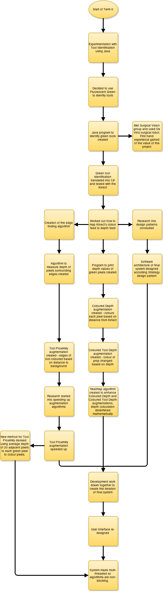
Development was roughly split into the following tasks:
  -Developing the green tool identification algorithm and early phases of development.
  -Developing the edge finding algorithm.
  -Learning to use the Kinect Coordinate Mapper.
  -Identifying green pixels and reading their depth.
  -Creating trivial versions of the ColoredDepth and ColoredToolDepth augmentations using depth thresholds to alter colour.
  -Creating the heat map algorithm to give advanced versions of the ColoredDepth and ColoredToolDepth augmentations.
  -Creating and speeding up the ToolProximity algorithm.
  -Creating and re-designing the final system.
  -Adding voice control functionality.
Below, each of these sections is documented to show their development as the project progressed. The completion of each of these tasks is considered a major technical achievement.

Development of the Green Tool Identification Algorithm and Early Phases of Development
At the start of the project one of the main issues that the team faced was how to identify the tool in the camera feed so that it could be visually augmented to give depth information back to the surgeon. Using advanced statistical techniques on the standard image was out of the question as that would have taken a considerable amount of time to implement, and the goal of this project was to provide depth information to the surgeon, not identify tools in the camera feed. The team had an idea at this point that would make identifying the tool extremely easy and simple, meaning we could focus on creating the system’s visual augmentations. The link below is to a slide deck that details early development and the conception of using fluorescent green to identify tools and the subsequent development of the algorithm used in the final system.

Tool Identification Development

Development of the Edge Finding Algorithm
Perhaps the most important augmentation included in the system is the ToolProximity augmentation, which changes the colour of a green tool in its view based on how close it is to the background. ToolProximity would let a surgeon know when their surgical tools are getting close to the body tissue.
In order to work out the distance between the tool and the background, the team decided that the easiest algorithm to implement would be find where the edges of the tool were, and then measure the depth values of the corresponding pixels and the pixels surrounding them. Of the surrounding pixels, some would be a part of the background, and could be identified as such because they were not green (which would mean that they were a part of the tool). Once this depth information was obtained, it was a simple matter to calculate the distance between the tool and the background.
In order to make that algorithm work, the surgical tool first needed to be identified (by looking for fluorescent green), and then the edges of it found. Finding the edges was the most critical part of this, as without knowing where the edges where the distance to the background could not be measured. Thus the edge detection algorithm was conceived.
The edge finding algorithm is used in the system to determine the edge of the tool so that the proximity of the tool to the background can be found. In simple terms the algorithm works by finding the green section of the image, then marks the edge of each section, thus producing an outline of the tool.

The first step on the road to creating the edge finding algorithm was the red removal program. This used a fairly simple algorithm which checked the red value of each pixel and set the pixel to black if above a certain threshold. At the time, the thinking behind this algorithm was that as most of the interior of the body is some shade of red, then by removing all of the red from the image the only thing left would be the tool. As it turned out, it wasn’t that simple and the team used the concept of bright green tools to identify them in the end. This simple algorithm would eventually led to the edge finding algorithm in the next iteration of development.

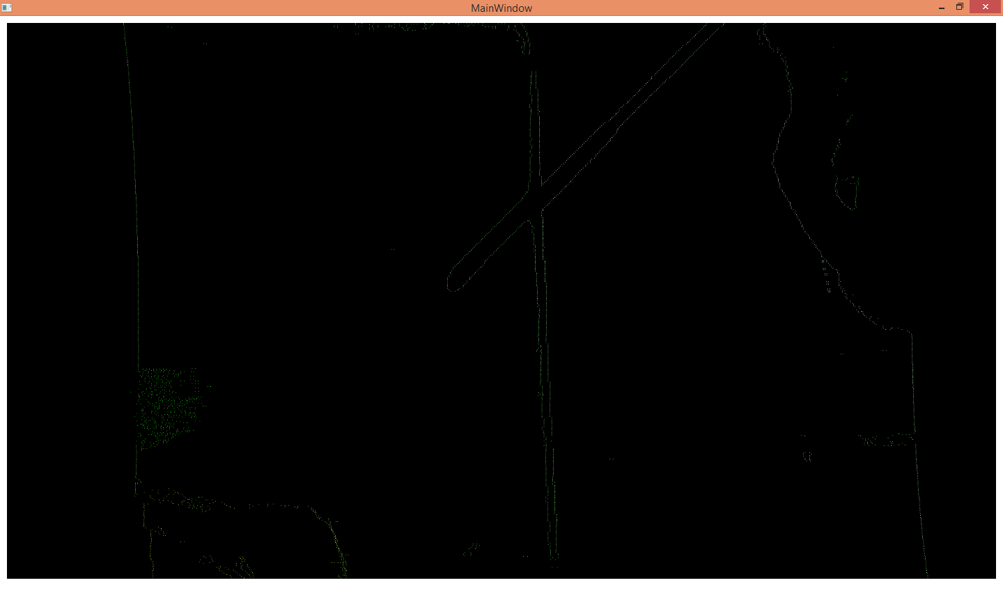
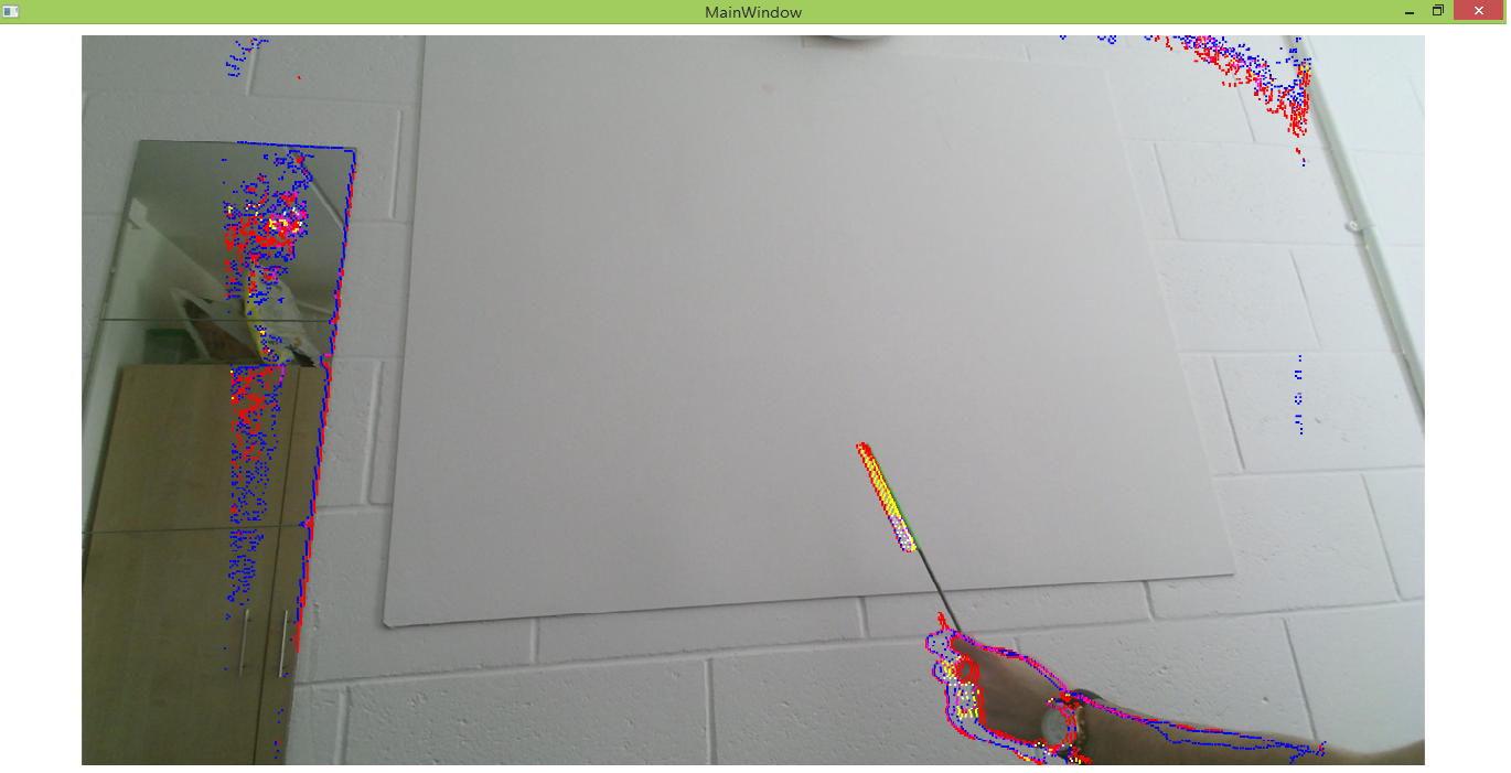
The first example of the edge finding algorithm was made in the next iteration of development. From the screenshot above it can be seen that there is too much noise in the image, but all of the edges, of the tool and the surrounding area, have been found. Further development is needed at this point because of the noise, however it is obvious to the human eye which part is the metal rod which is being used to simulate the surgical tool.

In the next iteration of development, a considerable amount of progress has been made. Much of the noise has been resolved, and the edges have been coloured according to how far away they are from their neighbouring pixels. However, this was achieved by conducting edge detection by change in distance to the background rather than searching for the edge of a green section, meaning that any edge in the picture, not just the green tool, were having the algorithm applied to them. This wasn’t acceptable for the final system as the algorithm would take too long to run if it worked in this fashion. It would need to be applied solely to the green sections of the image. Some noise also exists at the edges and in the mirror (which is unrealistic, you would not find a mirror in a human body, so can be ignored) exist and need to be removed.

In this final iteration of edge detection, green is searched for and then edge detection applied to the green section. Other objects can also be picked up if they have a high green content in them (such as skin) however since this is not visible in the body, where in fact much of the tissue is red, it should not be an issue. Therefore within the body this is a very good simulation for edge finding.
The edge finding algorithm was required to be able to find where we were going to check for proximity to the background in the ToolProximity augmentation. Without knowing where the edges were it would have meant we did not know where to check the distance to the background and as such we would not have been able to develop the ToolProximity augmentation, which was one of the main goals of the entire system, perhaps the most important of all.
Some possible future developments of the edge detection algorithm would be to explore other established algorithms which are more advanced than our own such as the Canny Edge Detection algorithm. At the time of development we felt it was best not to try and implement this algorithm until all other developments were concluded - we needed a basic edge detection algorithm that could be created fast, not a super-accurate one that took weeks to implement. As with tool identification, the project had to focus on depth sensing, not on algorithms to identify edges, so we needed to move on fast from creating an edge detection algorithm. The team decided to implement this algorithm if there was time after the final system was created instead.

Learning to Use the Kinect Coordinate Mapper
The Kinect sensor has two cameras in it, one standard colour camera and an infra-red camera which also measures depth. These cameras are beside each other in the Kinect unit, so the images received from each of them are slightly offset from each other. This can be seen in the photos below, in the depth image the radiator that is visible towards the right hand side of the colour image is not visible.

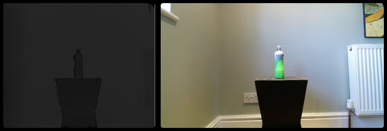
In this state, it is impossible to find out a depth value for any of the colour photo pixels because the depth and colour feeds do not line up. However, the Kinect SDK provides a CoordinateMapper class that will map each pixel of the depth image to the equivalent pixels in the colour image, meaning that each colour pixel will have an associated depth value.
It was essential that the team learn how to use this coordinate mapper, because we were going to need to identify tools by their green colour and then retrieve the depth values for each of these pixels. That meant that we needed to use both the colour and depth images, so would need to use the Coordinate Mapper.
To begin with we found this very complicated and struggled to get it to work. We eventually found that it only properly worked at a range of over a metre because at any distance less than this, the Kinect’s depth measurements were not completely accurate, which lead to some strange effects such as “doubling” of objects, where there would appear to be two of everything. Once we started experimenting with distances over a metre, the mapping worked well.
After testing that the coordinate mapper was working with some basic tests (described below and in the Testing section), the team developed a first iteration of the ToolProximity augmentation that relied on using the coordinate mapper. The goal here was to identify which pixel of the tool was closest to the background. We achieved this by conducting edge detection, mapping the depth and colour pixels, before checking each pixel’s neighbouring pixels and finally taking the maximum difference between the pixel that belonged to the tool and its neighbouring pixels.
After doing this for each of the pixels that belonged to the edge of the tool, the minimum value was found and the location of that pixel (in the image by x and y coordinates) was printed. By checking this with the standard colour picture which was also produced, we correctly managed to find the closest pixel to the background on most occasions, which we knew was correct as the tip of the rod was closest to the background and the identified pixel was mostly in this area of the picture. As a result we were confident with using the coordinate mapper for the remainder of the system.

Identifying Green Pixels and Reading Their Depth Values
One of the most important aspects of the development of the system was to check that the coordinate mapping function was working. It would be essential later in the project to retrieve the depth value of a pixel, based on what colour it was. This whole phase of development was effectively dedicated to testing whether this could be done.
The program written was relatively simple: it mapped the depth to the colour feed using the Kinect’s coordinate mapper, scanned through the image array looking for fluorescent green pixels (that belonged to a prop) and if it found them, printed the depth value for these pixel. It would be apparent that the coordinate mapper had worked correctly if the distance physically measured between the Kinect and the prop with a tape measure was equal to the depth values yielded by the Kinect. The following setup was used, with distance markers being placed at 30 centimetre intervals:

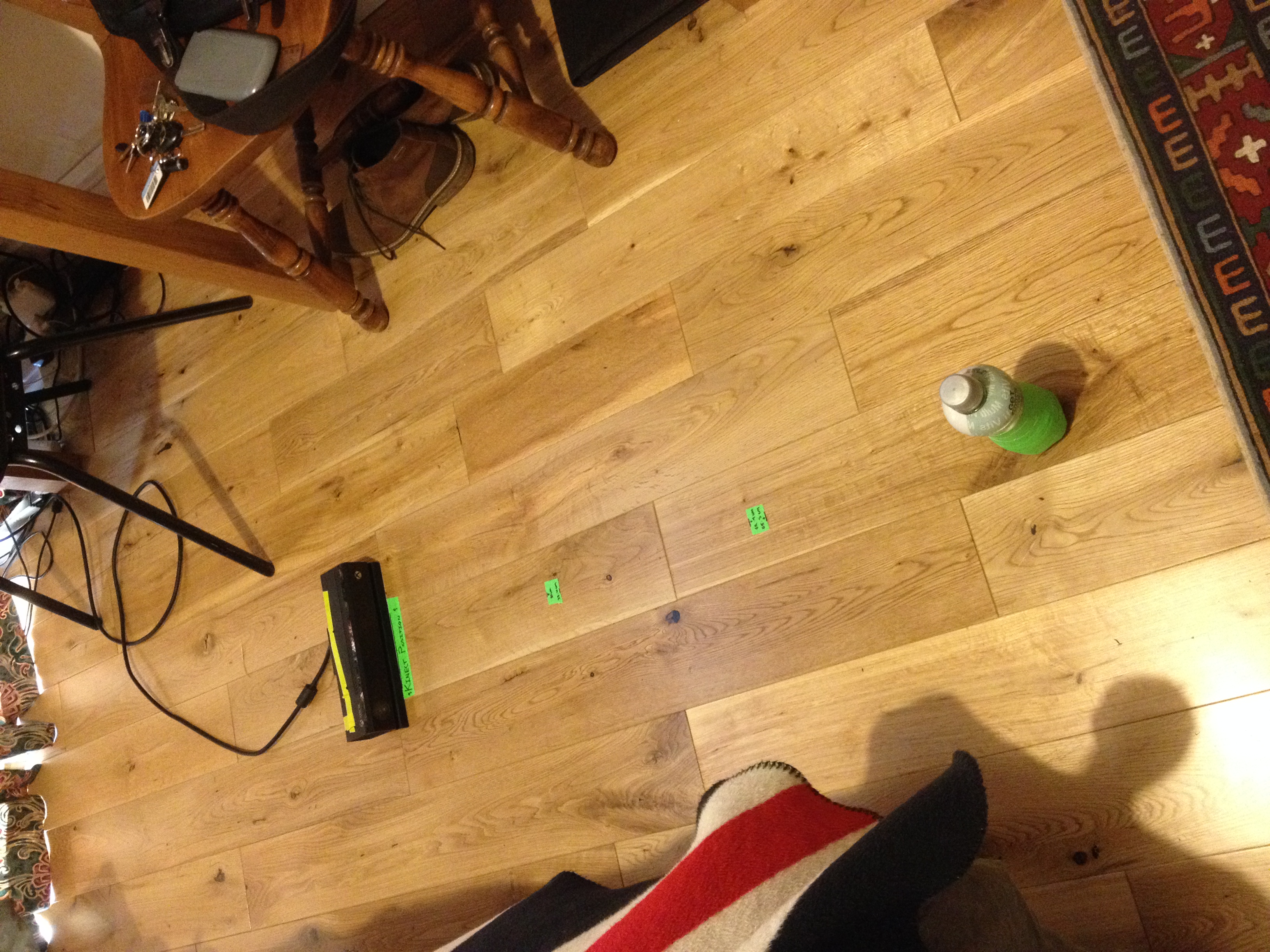
The prop (a bottle wrapped in green tape) was placed on the third distance marker approximately 93 centimetres from the Kinect as was physically measured. The algorithm was then started and the numbers yielded were in the range of 920 millimetres to 960 millimetres. The algorithm had therefore been a success, the variation likely due to the curvature of the bottle, with pixels with values such as 960 millimetres being further away from the Kinect along the curve of the bottle.
This test confirmed to us that the team had correctly used the Kinect’s coordinate mapper, which was a major achievement because the team had spent several weeks attempting unsuccessfully to use the coordinate mapper. Most importantly, the test confirmed that development could continue using the coordinate mapper in this way.

ColoredDepth and ColoredToolDepth First Iterations
Although the team considers ToolProximity to be the main and most useful augmentation of the system, it also created two others that could aid a surgeon in judging depth. These augmentations colour the whole image or just the tool respectively based on how far away it is from the camera. The use of this is that the surgeon can look at these views and get an intuitive feel for the 3D landscape of the surgical area.
The first step to creating both of these algorithms was to map the depth image to the colour so that each colour pixel had a corresponding depth value. The first iteration of the ColoredToolDepth algorithm would then scan through the colour image array and look for green pixels. When it found them, it would extract their depth value, and then set the pixel to a different colour based on its depth value. A threshold was used to do this, quite simply if the pixel was less than 700mm away from the Kinect it would be coloured red, less than 800 and it would be coloured orange and so on through yellow to green. The following screenshots show a prop being coloured according to these thresholds. The first photo is a normal one showing the test setup.

Although this algorithm sounds extremely simple, it taught the team a lot about the basic elements of displaying an augmented image.
When the coordinate mapper was tested by printing the depth values of green pixels, nothing was displayed on the screen. This meant that the team encountered a difficulty when attempting to display the augmented image - what size should the image array be? The same as the depth array or the colour array? The answer was neither.
The image array needed to be the size of four times the depth image array. This was because what we were effectively displaying using the image that had undergone coordinate mapping was the depth image as a colour image, as opposed to gray scale. Each pixel therefore required four bytes of data, for blue, green, red and alpha values (the depth values of each pixel were stored in a separate array). However the image was not as large as the colour image because the RGB camera is higher resolution than the depth camera, and the mapped image was the same resolution as the depth image. The team learned this while creating this first iteration of the ColoredToolDepth augmentation.
This test also highlighted the “doubling” issue that it was possible to get - in the augmented photos above you can see this effect taking place on the chair on which the bottle is stood. The issue turned out to be that if the Kinect was too close to the prop, then this doubling effect would be observed, so the prop just needed to be moved further away from the Kinect. It was lucky that the team caught this issue at this early stage, otherwise it could have turned out to be more of an issue at a later phase of development.

Tool segmentation using depth
In an actual, deployable system it would not be acceptable to identify tools by them being flourescent green. While this would make the whole task infinitely easier, it is unlikely that manufacturers of surgical equipment can be convinced to paint their tools flourescent green for the sake of a depth sensing system. It is therefore necessary to develop new ways of identifying the surgical tools in the camera feed.
The team has talked extensively with Max Allan from the Surgical Robot Vision Research Group at UCL about this issue and how the tool can be identified purely from the colour image (for full details, see the Surgical Vision Group Section of this website). However the techniques involved in doing this are extremely advanced, and would have taken a great deal of time to implement. The team could not afford to spend weeks identifying a tool by the colour image alone as the project needed to keep focused on depth sensing.
So instead, the team decided to try a different approach. This approach was to use the depth image to identify the tool, because the tool would most likely have a significantly different depth value than the surrounding background. Of course, this would not work when the tool was extremely close to or touching the background (such as the body in a surgical environment), but even in this case only the tip of the tool would be touching the background, the rest would still have a significant difference in depth to the background.
If the team could perfect this, then that would be excellent as a fully deployable tool identification algorithm would have been found. Even if the team only made a small amount of development with this, then this would still be extremely useful to future developers who may be looking to identify the tool by depth.
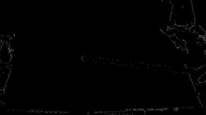
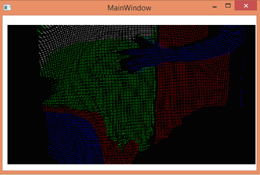
The team did this by finding edges based on depth, as this was sure to give the outline of the tool. The algorithm works by finding the difference between the depth of the current pixel and its neighbouring pixels. If the difference is above a set threshold then the pixel is identified as an edge of the tool. The main issue with this algorithm was that it slowed the performance of the system due to the huge amount of arithmetic functions it was performing.

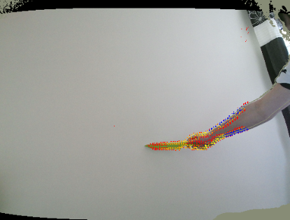
The above image illustrates the edge identification using the difference in the depth values. It finds the difference in the depth of the neighbouring pixels and determines if that pixel is an edge. As can be seen, all edges have been well identified, although of every object with an edge rather than just the tool.
The team did not progress much further than this with the development of an algorithm to identify tools by depth rather than colour because it was necessary to move on to the development of the final system, and identifying the tools by their green colour worked well enough for our purposes. However this would be one of the first objectives of any future development, as this algorithm shows huge potential.
For example if it was combined with recognition by colour techniques, it may make them far easier to implement as the pixels to look at could be identified by this algorithm finding the edges of the tools, and the identification by colour techniques could then only look at pixels between these edges to find the tool, perhaps increasing the efficiency of the identification algorithm by a great deal. Needless to say, this should be one of the first areas of development that future developers look to work on.

ColoredDepth and ColoredToolDepth using the Heat Map Algorithm
The previous iteration of the ColoredDepth and ColoredToolDepth augmentations used simple depth thresholds to colour the image. While this worked well enough, the team knew of the existence of algorithms that would assign each pixel a colour based on its depth, which would give a much nicer looking image for these two augmentations than simply using thresholds. The algorithm the team use is called a heat map.
A heat map is a graphical representation of data where individual values contained in a matrix are represented as colors. The ColoredDepth view of the depth sensing endoscope makes use of a heat map. The heat map is generated depending on the pixel’s distance away from the Kinect (i.e. its depth depth). This would provide the surgeon with a coloured depth view that would help them judge the distance of the tool from the body. The colour of the tool changes as the tool gets further away from the camera.
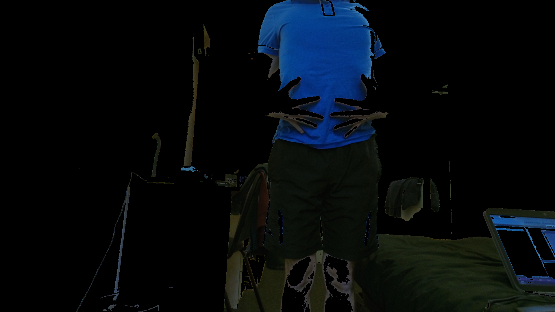
The initial prototype of the ColoredDepth augmentation was based on rigid thresholds. If the depth of the object were in a provided range the object would be displayed in a distinctive color. However, the problem with this prototype was the absence of gradual continuity in terms of color change of the object based on depth. The depth segmentation using rigid threshold is illustrated below:

This shows the feed segmented based on its depth. The depth value of the pixels are analyzed and the color is set based on the depth range. This implies that a range of depth values correspond to the same color and hence there is no gradual demarcation in depth and the depth values are not exploited to their maximum capacity. The hand in the image is closer to the camera and hence is blue.

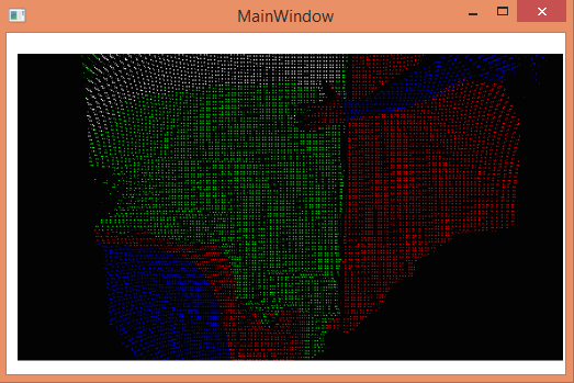
The above image depicts that as the hand moves away from the camera it turns red. The background appears in green and white. The varying depths of the background cannot be demarcated as all the depths in a particular range have a specific color and not a range of colors. There is no gradual continuity in the color view using the depth values when using this thresholding technique.
The final prototype was to develop an algorithm that would provide the gradual and more sophisticated change in the color of the object. An example of the functioning of the heat map was illustrated to us by PhD student, Aron Monszpart. The heat map was then implemented as it was a more sophisticated approach towards depth colouration than segmentation by rigid thresholds.
The heat map algorithm attains the rightmost 8 bits of the depth value of each pixel. To convert to a byte, the most-significant bits are discarded rather than least-significant bits. The bitwise “and” operation provides with the right-most bits. Based on the depth value the color spectrum is chosen and the color values are assigned based on the right-most bits of the depth value. This provides continuity in the color spectrum of the field.

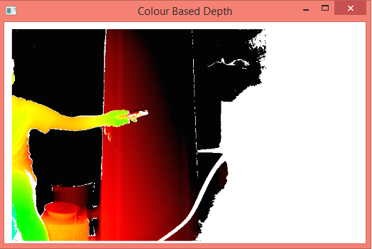
The above image illustrates the final heat map designed for the system. The heat map provides a gradual continuity in the color spectrum using the depth values. This provides more extensive information of the depth as it changes the shade of the color as it moves to and from the camera.
This algorithm can identify the most minute differences in depth between each pixel, meaning the the surgeon, when looking at this image, can get a very good idea of the three-dimensional layout of the image they are seeing. This would be extremely useful in surgery, for example if the surgeon were looking at two blood vessels and could not tell which one was closer on the 2D image, they could simply turn on the ColoredDepth augmentation and instantly it would be obvious which vessel were closer. If a rigid thresholding system were being employed, then both vessels may be in the same threshold so difficult to tell apart, but with heatmap algorithm it is easy to tell the smallest differences in depth, which is what makes this augmentation so valuable.

Creating and Optimising the Tool Proximity Algorithm
The tool proximity algorithm is perhaps the most important augmentation of the system. It informs the user when a tool is getting close to the background by changing the colour of the tool’s edges, meaning it could tell a surgeon when their tools are getting close to the body tissue. On a high level, it works by using the edge finding algorithm to find the edges of the tool before searching the difference in distance from the tool to the background. The edges are then coloured a certain colour depending on the scale of this distance, with red implying close proximity, to blue implying the distance is large.
Initially we intended to segment the tool by using depth segmentation, in other words finding large changes in depth and accepting that as an edge of the tool. This did not work properly for two main reasons: firstly when the tool was touching the background, that section of the tool was impossible to segment as it would effectively blend into the background. In addition, since the mapping was not 100% accurate there was often a ±5 pixel difference between the depth and colour images meaning the augmentation was not always correctly placed. This is seen in the image below where the augmentation is approximately 3 pixels to the left of where it should be.

The other main issue was the amount of noise which was picked up simply from fairly flat surfaces, since any change in depth would be seen as a tool edge. In order to overcome this problem we decided to search the image for a green section as we knew that the tool would be coloured green. From this, the edges of the green section could be mapped onto the depth map in order to find the proximity of the tool to the background.
Another reason for the change in approach for segmenting the tool was due to the fact that the augmenter was running very slowly as it was algorithmically intensive. As a result the system was running at less than 1 frame per second at times. It goes without saying that this is unacceptable for surgery as it would be impossible to see what was happening. By only applying the edge detection algorithm to green sections of the image, the process was greatly speeded up, although further work was still required to be able to produce a truly fast frame rate. By changing the approach, the positioning of the augmentation was also perfect since it was the green pixels which were sought out. This is seen in the image below.

In order to present the proximity of the tool to the background, each pixel at the edge of the tool would be coloured, with red being the closest, through to orange, yellow and then blue being further away. As this system is a larger than scale simulation, any distance under 1 centimetre is not coloured otherwise the amount of noise would be too large. In terms of the simulation, a 1 centimetre tolerance is a reasonable distance since this is still sufficiently close to the background, and when scaled down for actual surgery that distance would be negligible as an actual depth sensor in a surgical environment would be extremely accurate over short distances, which the Kinect is not.
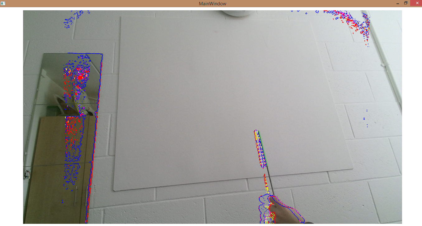
During the testing phase of the system, it became apparent that this version of the ToolProximity augmentation still needed some development. This is because the image produced when colouring just the edges of the tool was extremely granular and potentially fairly noisy. This is shown in the image below:

This image is fairly confusing, because in the innermost ring of colour on the green bottle, the pixels are coloured orange and red, but further out on the bottle, around its actual edges, the pixels are coloured yellow. This is could be confusing to users trying to judge the depth of the tool.
To rectify this issue, the ToolProximity algorithm was modified to use a slightly different technique. This technique was that at each green pixel found in the image, the depth of the twenty pixels directly adjacent to it were gathered and then averaged, and the green pixel then coloured according to the average depth of those pixels adjacent to it. This algorithm allowed the whole green area of the tool to be coloured, not just its edges. The whole tool would then move through a spectrum of green, yellow, orange and red as it got closer to the background, with red signifying that the tool was about to touch the background. Images of this are shown below.

The first of these images shows all of the colours of the distance spectrum, green through to red. The different sections are all coloured differently because the prop (green bottle) in the image is tilted towards the Kinect, so that the different parts of its body are different distances from the background. In the second image, the bottle is held flat against the background (the wall) and thus is completely red because it is touching the background.
This algorithm is far less precise than the previous iteration of the ToolProximity augmentation because it does not measure the depth of pixels directly next to the pixels that form the edges of the tool, but takes an average of the twenty adjacent pixels to every green pixel. Both versions of the ToolProximity augmentation have great potential, but the first version that uses edge detection needs more development to reduce noise and the granularity of the coloured pixels before it can be used.
It is worth noting that the ToolProximity algorithm is best used to monitor when a tool is getting close to the main component of the background, not to lesser components. What this means is that in a surgical scenario this augmentation would be used to monitor a cutting tool as it moved towards a layer of tissue that it was going to cut through, and would be useful because it would tell the surgeon when the tool is getting close so they should apply less force to it so they do not accidentally cut the patient.
This augmentation would not be used if the surgeon was trying to pass a piece of string around a blood vessel (called “slinging” a blood vessel) and was trying to judge how close their tools were to the blood vessel. This is because the method of taking an average of the twenty pixels adjacent to each tool pixel would read the depth values of the main background tissue more than it would read depth values of the blood vessel, meaning the tool would be coloured according to how far away it is from the background body tissue, and not the blood vessel.
However, if the ToolProximity algorithm that makes use of the edge detection algorithm was perfected, then it could be used for that process, because the edges of the tool that are over the blood vessel would have the distance to the blood vessel measured, not an average distance, so would tell when the tool was getting close to the vessel. This augmentation will need more development before it is capable of this however.

Creating and Re-Designing the Final System
The final system was what drew all of the the augmentations that had been created together to create a proof of concept system, proving that this depth sensing technology has a place in surgery. This primarily involved the creation of the UI, and the implementing of the Strategy design pattern according to the architecture that was previously designed.
Much of the experimental and research work that the team did with the Kinect was done by adapting the example programs provided with the Kinect such as ColorBasics and DepthBasics. Adapting these meant that the team did not have to deal with setting up the UI and working out how to actually display an image on the screen, because this was all handled by the example program; we would just alter the image which the example framework would then display.
However, it was not possible to adapt another program for the final system, we would have to build it from scratch. That meant that the team needed to learn exactly how you took a byte array and turned it into an image. Working this out was not a particularly hard task, and was done by simply working slowly through the example programs and commenting out various lines of code to see what would happen and what they did. Eventually the team had a good understanding of how to take the image array we were left with after applying the augmentation and display it on the screen.
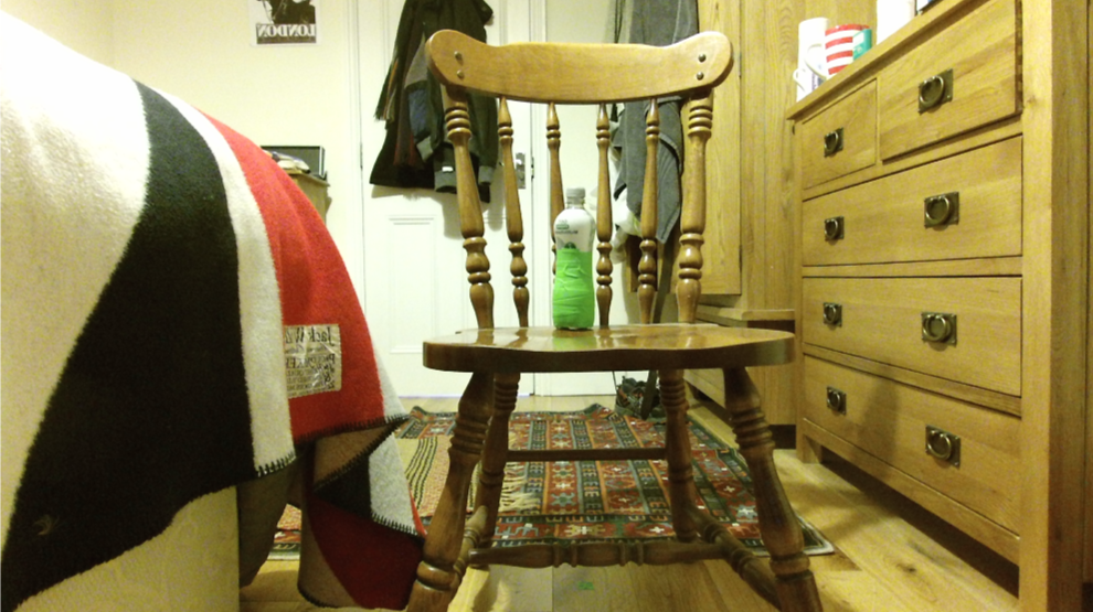
With each of the examples provided, only a single feed from the Kinect ever seemed to be used - either the depth or the colour. The team would however need to use both feeds in the system, so needed to find out how to receive both feeds from the Kinect at the same time. After conducting some research, the team discovered the multi-source frame reader, which allowed more than one feed to be received from the Kinect at any one time. To test the multi-source reader, a small program was created from scratch which displayed the colour and depth images side by side:

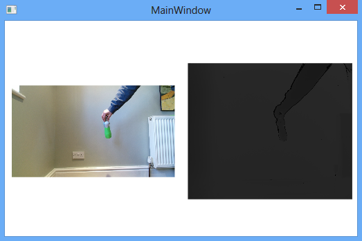
As can be seen, the prop, in this case a bottle wrapped in green tape, is shown in both the colour and depth images, both of which were received from a multi-source reader. Building this small experimental program was a very valuable task for two reasons: It taught the team how to use the multi-source reader. It was built from scratch, so showed the team how to build Kinect enabled applications, including the user interface, from a blank project which would be necessary for the construction of the final system.
Experimentation of writing Kinect enabled applications from scratch largely stopped after this point until the construction of the final system, because the augmentations had to be created and the architecture of the system designed. Once these things had been done, it came time to create the final system proper.
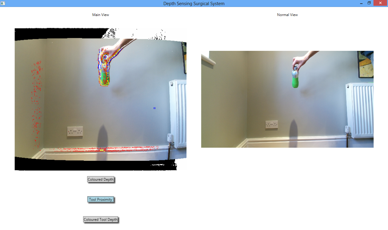
The team originally intended to follow our UI designs from the previous term precisely (link to PDF of UI design goes here), however realised that this would be a foolish thing to do when it came to building the system. This was because if the augmentations were to malfunction or run slowly, then it was important the surgeon have a backup view of the operational area so that they never lose sight of what they are doing, as this could be extremely dangerous for the patient. The team therefore decided that the final system would have three separate views, one for the augmentation, one normal view with no augmentation whatsoever, and a simple gray scale depth view. This would make it easy to see the differences that our augmentation was making for the purposes of demonstration, but more importantly in surgery would ensure that the surgeon never loses sight of the surgical area if one of the augmentations malfunctions, because there would at all times be a normal, unaugmented feed shown beside the augmented view. This is what the first iteration of the final system looked like:

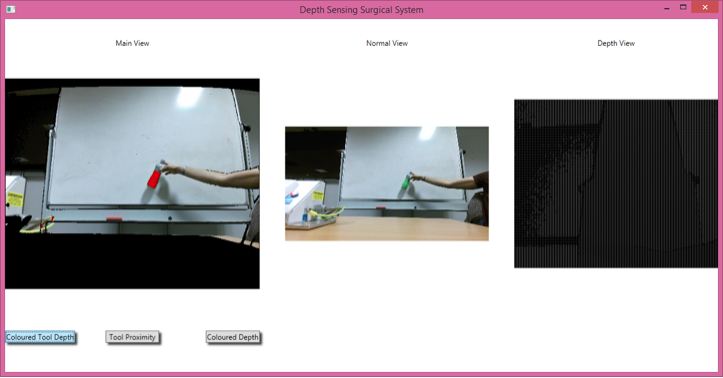
The augmentation is displayed in the “Main View” section of the system towards the left hand side of the image. The normal view is then displayed in the middle and the depth view on the right hand side. The issue with this interface is that all of the views are relatively small, which is not a good design for a surgical system as a surgeon would need the image to be large so that they could see detail in it, which is difficult with a smaller view. Furthermore, the depth view is utterly useless here as almost nothing can be discerned on it given that it is a gray scale image.
The team decided to redesign the interface, with focus on larger views and getting rid of the depth view. The result was this:

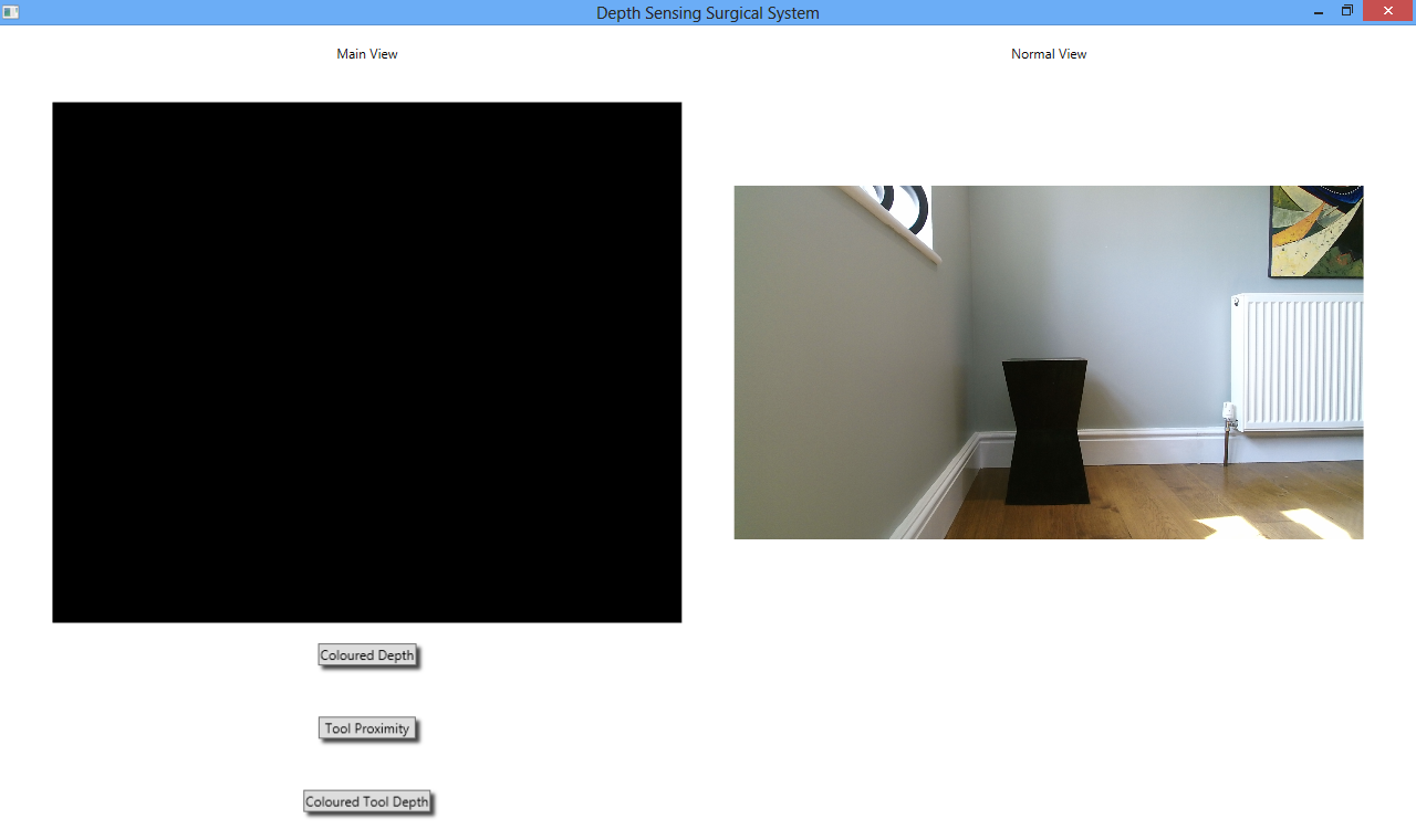
The augmentation view is again on the left hand side of the image and the normal view on the right. There are currently no augmentations being applied to the feed, so the augmentation view is blank. This interface is far more suitable for a surgical environment than the previous design for several reasons.
Firstly both views are much larger than they were in the first version of the final system, which would provide the surgeon with a much better view of the operational area than previously. Secondly the interface looks far less cluttered now that the depth view has been removed. Having both views displayed side by side is a particularly important design feature here, because it acts as a failsafe mechanism. If the augmentation being displayed in the left hand view were to freeze or run incorrectly in any way and it was the only view being shown, then there could be a danger to the patient because the surgeon would not be able to see what they were doing. However because there is a normal view displayed at all times next to the augmented view, if the augmented view fails the surgeon will still be able to see the normal view so can monitor what is going on inside the patient’s body, reducing the risk to the patient.
The team was now satisfied with the interface design for the system, but had run into a serious issue when beginning to test it. This issue was that the augmentation algorithms ran far more slowly than the frame rate provided by the Kinect, meaning that the system would constantly freeze and crash for both the normal view and the augmented view. Clearly, this was completely unsuitable for surgery because it would be extremely dangerous for the patient if the system crashed and froze constantly.
The team knew that it was the slow speed of the augmentation algorithms running that caused this, so employed another important design feature by running the augmentation algorithms in a separate thread of execution to the button click event handlers and the normal view.
Doing this greatly improved the system, the augmentations now ran much faster but most importantly the issue of freezing and crashing was stopped. The normal view, since it runs in a different thread to the augmentation view, always displays a realtime view of what is happening, regardless of whether the augmentation view is running slowly or not. The buttons are guaranteed not to freeze either because they also run in a separate thread to the augmentation.
Standard thread safety techniques were used in the implementation of this. The augmented image array is actually displayed by the main thread, but is updated by the augmentation thread. It was the updating of the augmented image by the augmentation algorithm that was previously causing the problem, not the displaying of the actual image. This however means that the augmented image array is accessed by both threads of the system, which could yield synchronisation issues. To protect against this, the augmented image array object is declared “volatile” so that it is flushed to memory after every alteration by the augmentation thread, so the most up-to-date version of the array is always accessed by the main thread to be displayed.
Images of the various different augmentation running on the final system can be seen here:

Final System In Action

Adding Voice Control Functionality
When it came to designing a way to control the Depth Sensing Surgical System, the team had to bear several things in mind. The first of these was that it must be quick and easy for the surgeon to switch between different augmentations because they will be concentrating on the surgery they are performing and cannot waste time trying to understand the system; it must be intuitive. The second was that the surgeon would be scrubbed up, meaning that they would not be able to touch physical controls for the system, unless these were on the laparoscope itself. The solution the team devised was to use voice control. (For full documentation of the design of the system controls, see the link here).
Having voice control would allow the user to switch between the different augmentations that the system has to offer without physically pressing a button. This means that when the surgeon is scrubbed up, they will be able to change the augmentations being shown simply by speaking their names rather than getting an assistant to press a physical button or click a different option on the endoscope terminal.
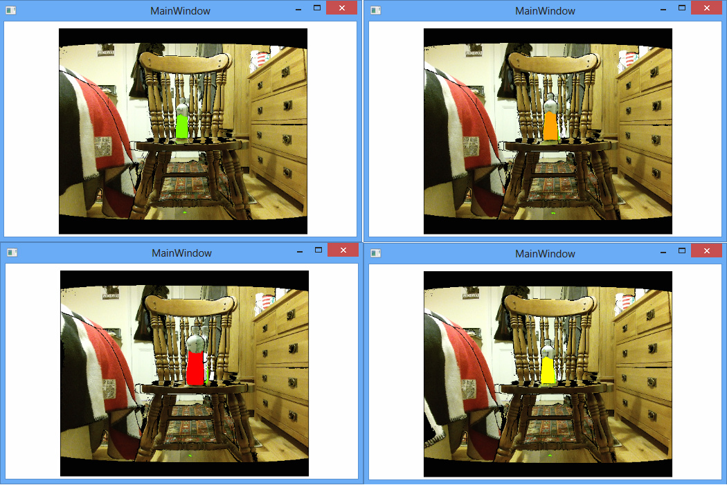
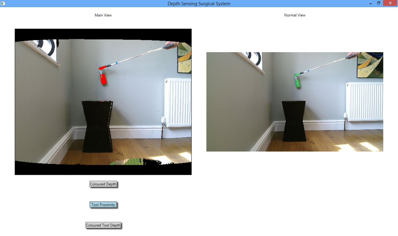
The system provides three different augmentations: ToolProximity, ColoredDepth and ColoredToolDepth that the user can switch between with voice control. The speech recognition ability of the Kinect was exploited for this purpose. Speech recognition is one of the key functionalities of the NUI (Natural User Interface) API. The Kinect sensor’s microphone array is an excellent input device for speech recognition-based applications.
The speech recognition algorithm runs as follows: the grammar for the voice control is set, and the commands can then turn on and off the different views available. The Kinect speech recognizers are then initialized. When a SpeechRecognized event is encountered a “confidence threshold” value is set. This value gives the application a way to specify its level of confidence in what was spoken: 1% means that the speech recognition engine completely lacks confidence in what was spoken, and 100% means that it is completely confident. When the appropriate voice command is spoken the respective augmentation is turned on.

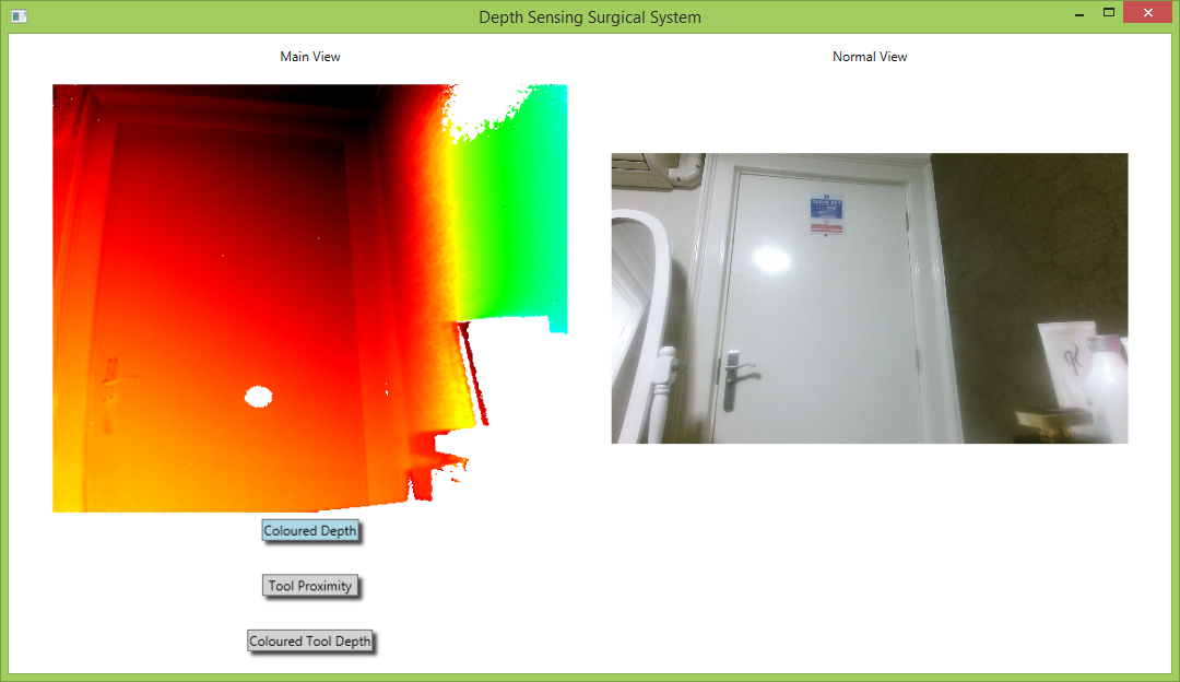
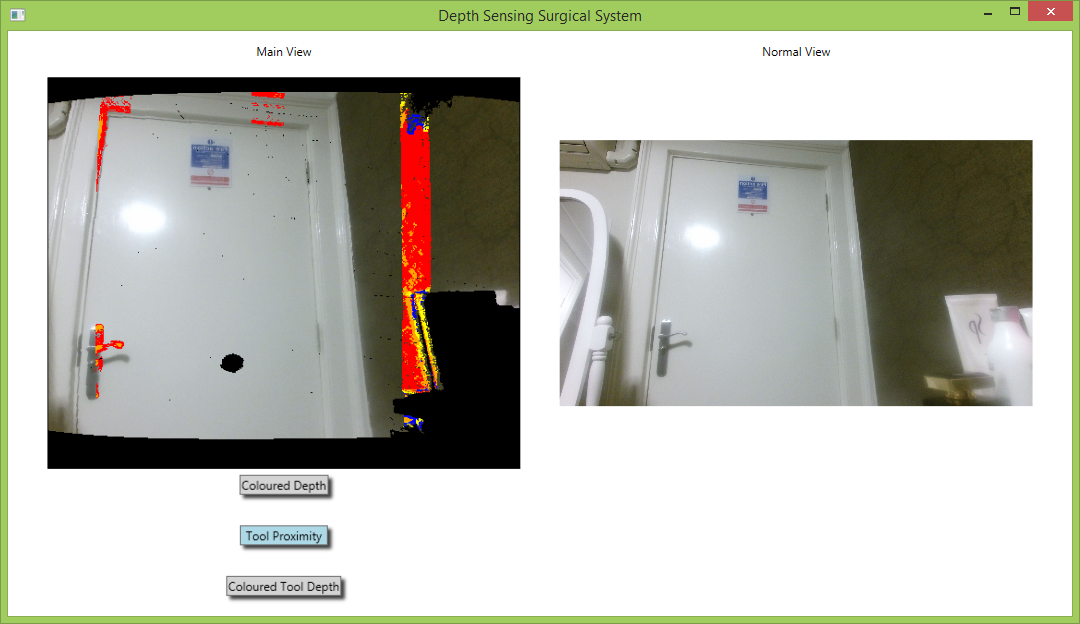
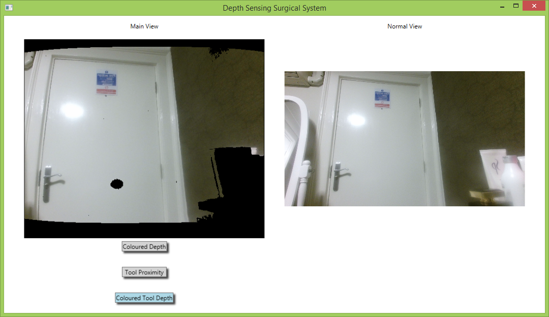
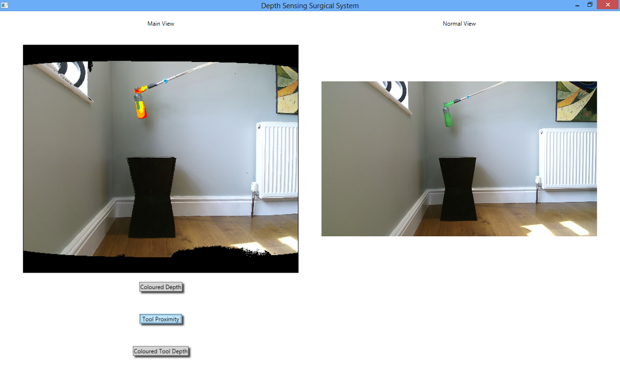
The above images illustrate the voice control functionality. The first image depicts the system view when the command “Colored Depth On” was uttered. The second image depicts the system view when “Tool Proximity On” was uttered, and the third depicts the view when “Tool Depth On” was uttered.